|
|
 |
Fiche d'espèce de Copépode |
|
|
Calanoida ( Ordre ) |
|
|
|
Clausocalanoidea ( Superfamille ) |
|
|
|
Clausocalanidae ( Famille ) |
|
|
|
Clausocalanus ( Genre ) |
|
|
| |
Clausocalanus arcuicornis (Dana, 1849) (F,M) | |
| | | | | | | Syn.: | Calanus arcuicornis Dana, 1849;
Clausocalanus arcuicornis major : Tanaka, 1956 c (p.383, fig.11a: F); Mulyadi, 2004 (p.182, figs.M, Rem/no Dakin & Colefax, 1940 (p.97, figs.F);
Clausocalanus sp. : Grandori, 1910;
no C. arcuicornis : Esterly, 1905 (p.142, figs.M); Sewell, 1929 (p.90, Rem.: 2 forms); Mori, 1937 (1964) (p.54, figs.F); Tanaka, 1937 part. p.252, fig.2, a, c,: F large specimen); Ramirez, 1966 (p.10, figs.F,M); Park, 1968 (p.541, figs.F); Bradford, 1972 (p.36, figs.F,M); Williams & Wallace, 1975 (p.176, fig.F);
Clausocalanus arcuicornis var. plumulosus: Sewell, 1913 b (p.367); Silas, 1972 (p.646)
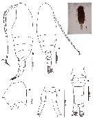
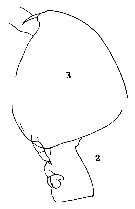
Clausocalanus brevicornis : Acha & al., 2020 (p.1, Table 3: occurrence % vs ecoregions) [probably lapsus calami; C.R.]. | | | | Ref.: | | | Giesbrecht, 1892 (part., p.186, Pl. 10, figs.8, 16, 19; Pl. 36, fig.30); Wheeler, 1901 (p.171, figs.F,M); Thompson & Scott, 1903 (p.233, 244); ? Farran, 1908 b (p.28); ? A. Scott, 1909 (p.32); ? Wolfenden, 1911 (p.203); Sewell, 1912 (p.360); 1914 a (p.214); ? With, 1915 (p.68, figs.F); Früchtl, 1923 a (p.139, 140, figs.F); Früchtl, 1924 b (p.20, 43, fig.F); Sars, 1925 (p.27); Farran, 1926 (part., p.237); Candeias, 1926 (1929) (p.30, figs.F); Farran, 1929 (part., p.208, 223); Rose, 1929 (p.17); ? Wilson, 1932 a (p.42, figs.F,M); ? Rose, 1933 a (p.81, figs.F,M); ? Farran, 1936 a (part., p.80); Tanaka, 1937 (part. p.252, fig2, b, d, Rem., small specimen); Lysholm & al., 1945 (p.10); Vervoort, 1946 (p.140, Rem.); Sewell, 1947 (part., p.54); 1951 (p.357, 389, Rem.: parasites); ? Brodsky, 1950 (1967) (p.118, figs.F,M); Vervoort, 1957 (part., p.37, Rem.); Marques, 1958 (p.208); Tanaka, 1960 (Pl. X, figs. 2, 3, data from Frost & Fleminger); Heinrich, 1961 b (p.93); Vervoort, 1963 b (p.117, Rem.); Chen & Zhang, 1965 (p.49, figs.F,M); Marques, 1973 (p.237); Unterüberbacher, 1964 (part., p.19, figs.F); Owre & Foyo, 1967 (p.41, figs.F,M); Frost & Fleminger, 1968 (p.46, figs.F,M, Rem.); Corral Estrada,1970 (p.140, figs.F, Rem.); Razouls, 1972 (p.94, Annexe: p.34, figs.F); Chen & Zhang, 1974 (p.103); Dawson Knatz, 1980 (p.7, figs.F,M); Alvarez-Marques, 1981 (p.157, figs.F, Rem.); Gardner & Szabo, 1982 (p.180, figs.F,M); Rudyakov, 1982 (p.209); Brodsky & al., 1983 (p.230, figs.F,M, Rem.); Van der Spoel & Heyman, 1983 (p.44, fig.56); Zheng Zhong & al., 1984 (1989) (p.235, figs.F,M); Lin & Nakamura, 1993 (p.449); Bradford-Grieve, 1994 (p.109, figs.F,M, fig.101); Chihara & Murano, 1997 (p.776, Pl.91,94: F,M); Hure & Krsinic, 1998 (p.100); Bradford-Grieve & al., 1999 (p.878, 916, figs.F,M); Bucklin & al., 2003 (p.335, tab.2, fig.1, Biomol.); Conway & al., 2003 (p.181, figs.F,M, Rem.); G. Harding, 2004 (p.45, figs.F,M); Boxshall & Halsey, 2004 (p.93: figs.F); Blanco-Bercial & Alvarez-marqués, 2007 (p.73, fig.2, Biomol.); Avancini & al., 2006 (p.75, Pl. 44, figs.F,M, Rem.); Vives & Shmeleva, 2007 (p.614, figs.F,M, Rem.); Phukham, 2008 (p.128, figs.F); Blanco-Bercial & al., 2011 (p.103, Table 1, Biol. mol, phylogeny); Blanco-Bercial & al., 2011 (p.108, fig.2, phylogeographic biomol. analysis); Blanco-Bercial & al., 2014 (p.6, Rem.: problematical for barcoding) | 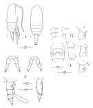 issued from : B. Frost & A. Fleminger A. in Bull. Scripps Inst. Oceanogr. Univ. California, San Diego, 1968, 12. [Pl.29, p.158-159; Pl.30, p.160-161; Pl.31, p.162-163]. Female: 1 a, habitus (right lateral view); 1 b, idem (dorsal view); taken from different specimens; 2 a-d, rostrum (right lateral view); 2 e-f, rostrum (anteroventral); 2 g-i, Th.4-5 (posterior part) and genital segment (right lateral); j, genital segment (ventral view); 2 k, B2 of P2; 2 l, B2 of P3; a-j taken from different specimens; k-l from one specimen; 3 a, Th.4-5 (posterior part) and urosome with spermatophore attached (right lateral); 3 b, Re3 and St of P3; 3 c-d, P5; taken from different specimens.
|
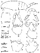
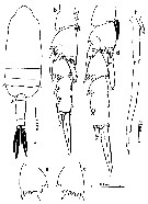
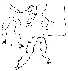
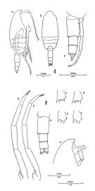 issued from : B. Frost & A. Fleminger in Bull. Scripps Inst. Oceanogr. Univ. California, San Diego, 1968, 12. [Pl.32, p.164-165; Pl.33, p.166-167]. Male: 1 a, habitus (right lateral view); 1 b, idem (dorsal view); 1 c, Th.4-5 (posterior part) and urosome (right lateral); taken from different specimens); 2 a, frontal region of C-Th1 (right lateral view); 2 b, urosome (dorsal); 2 c-d, B2 of P2; 2 e-f, B2 of P3; 2 g, P5 (posterior); 2 h, P5 (right posterolateral; a-b : taken from different specimens; c, f, h: from a third specimen; d, e, g: from a fourth specimen. Nota: Prosome less than 5.7 times as long as urosomal segment 2.
|
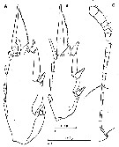
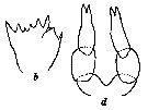
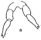
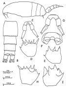 issued from : C. Razouls in Thèse Doc. ès Sciences, Univ. P & M. Curie, Paris , Tome annexe, 1972, Fig.34 (unpublished). Female (from Banyuls): A, habitus (lateral left side); B, urosome (dorsal); C, G, P5 (from different specimens); D, basipod 2 of P2; E, basipod 2 of P3; F, genital complex (ventral view); H, basipod 2 of P2; I, basipod 2 of P3.
|
 issued from : C. Razouls in Thèse Doc. ès Sciences, Univ. P & M. Curie, Paris , Tome annexe, 1972, Fig.35 (unpublished). Female (from banyuls): A, exopod 3 of P3; B, exopod 3 of P2; C, A1.
|
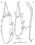
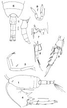 issued from : F.C. Ramirez in Bol. Inst. Biol. Mar., Mar del Plata, 1966, 11. [Lam.II, Figs.1-8] Female (from off Mar del Plata): 6, habitus (dorsal and lateral right side); 7, distal edge of basipodite of P2; 8, P5. Male: 1, habitus (dorsal); 2, urosome (posterior part cephalothorax with P5 and urosome (lateralright side); 3, P2; 4, distal edge of basipodite and endopodite of P3; 5, P5.
|
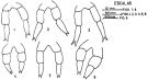 issued from : J. Corral Estrada in Tesis Doct., Univ. Madrid, A-129, Sec. Biologicas, 1970. [Lam.40, figs.1-6]. Female (from Canarias Is.): P5 from different individuals of different size: 1, 1.13 mm; 2, 1.20 mm; 3, 1.27 mm; 4, 1.33 mm; 5, 1.38 mm; 6, 1.47 mm.
|
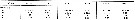
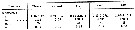 issued from : B. Frost & A. Fleminger in Bull. Scripps Inst. Oceanogr. Univ. California, 1968, 12. [p.46, Table 3a]. Clausocalanus arcuicornis Females: Measurements and ratios. TL = total body length ; SL = spermatophore length ; P :U = ratio of prosome length to urosome length ; U :U1 = ratio of total urosome length to length of 1st urosomal segment (genital segment) ; S :U1 = ratio of spermatophore sac length to U1 length of female on which spermatophore is attached ; r = sample range; m = sample mean; n = number of specimens measured; s = sample standard deviation.
|
 issued from : B. Frost & A. Fleminger in Bull. Scripps Inst. Oceanogr. Univ. California, 1968, 12. [p.47, Table 3b]. Clausocalanus arcuicornis Males: Measurements and ratios . TL = total body length; P :U = ratio of prosome length to urosome length ; P:U2 = ratio of prosome length to length od 2nd urosomal segment; U2:2P5 = ratio of U2 length to length of 2nd segment of longer ramus of P5; U2:3P5 = ratio of U2 length of 3rd segment of longer ramus of P5; 3P5:2P5 = ratio of length of 3P5 of longer ramus to length of 2P5 of longer ramus; r = sample range; m = sample mean; n = number of specimens measured; s = sample standard deviation.
|
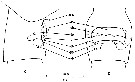 issued from : B. Frost & A. Fleminger in Bull. Scripps Inst. Oceanogr. Univ. California, 1968, 12. [p.104, P1.2, a, b]. Female: a, posterior part of last thoracic segment and genital segment (right lateral); b, genital segment (ventral). 3P5 = 3rd segment of P5; p = genital plate; cb = chitinous bar connecting seminal receptacles; lp = lateral edge of genital plate; s = edge of sternum overlying genital plate; dl = dorsal lobe of seminal receptacle; gp = region of genital pore; vl = ventral lobe of seminal receptacle. In illustrations genital segments, internal structures are outlined with solid lines in lateral view and with broken lines in ventral view.
|
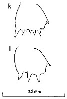 issued from : B. Frost & A. Fleminger in Bull. Scripps Inst. Oceanogr. Univ. California, 1968, 12. [p.161, Pl.30, k, l]. Female: k, basipodite 2 of P2; l, basipodite 2 of P3.
|
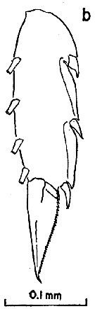 issued from : B. Frost & A. Fleminger in Bull. Scripps Inst. Oceanogr. Univ. California, 1968, 12. [p.163, Pl.31, b]. Female: b, exopodal segment 3 and terminal seta of P3.
|
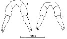 issued from : B. Frost & A. Fleminger in Bull. Scripps Inst. Oceanogr. Univ. California, 1968, 12. [p.163, Pl.31, c, d]. Female: c-d, P5 (from different specimens).
|
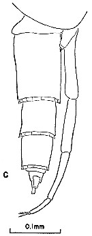 issued from : B. Frost & A. Fleminger in Bull. Scripps Inst. Oceanogr. Univ. California, 1968, 12. [p.165, Pl.32, c]. Male: c, posterior part of last thoracic segment and urosome (right lateral).
|
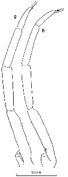 issued from : B. Frost & A. Fleminger in Bull. Scripps Inst. Oceanogr. Univ. California, 1968, 12. [p.167, Pl.33, g, h]. Male: g, P5 (posterior); h, P5 (right posterolateral, from another specimen).
|
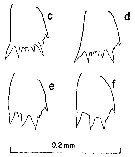 issued from : B. Frost & A. Fleminger in Bull. Scripps Inst. Oceanogr. Univ. California, 1968, 12. [p.167, Pl.33, c-d, e-f]. Male: c-d, basipodite 2 of P2; e-f, basipodite 2 of P3.
|
 issued from : C. Razouls in Th. Doc. Etat Fac. Sc. Paris VI, 1972, Annexe. [Fig.34]. Female (from Banyuls, G. of Lion): A, habitus (lateral); B, urosome (dorsal); C, P5; D, basipod 2 of P2; E, basipod 2 of P3; F, spermatheque; G, P5 (another specimen); H, basipod 2 of P2 (idem); I, basipod 2 of P3 (idem).
|
 issued from : C. Razouls in Th. Doc. Etat Fac. Sc. Paris VI, 1972, Annexe. [Fig.34]. Female: A, exopod 3 of P3; B, exopod of P2; C, A1.
|
 issued from : G. Harding in Key to the adullt pelagic calanoid copepods found over the continental shelf of the Canadian Atlantic coast. Bedford Inst. Oceanogr., Dartmouth, Nova Scotia, 2004. [p.45]. Female & Male.
|
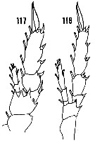 issued from : H.B. Owre & M. Foyo in Fauna Caribaea, 1, Crustacea, 1: Copepoda. Copepods of the Florida Current. [p.26, Figs.117-118]. Female: 117, P3; 118, P4.
|
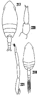 issued from : H.B. Owre & M. Foyo in Fauna Caribaea, 1, Crustacea, 1: Copepoda. Copepods of the Florida Current. [p.41, Figs.217-218, 220-221]. Female: 217, habitus (dorsal); 220, P5. Male: 218, habitus (dorsal); 221, P5.
|
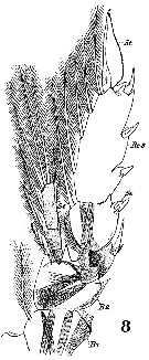 Issued from : W. Giesbrecht in Systematik und Faunistik der Pelagischen Copepoden des Golfes von Neapel und der angrenzenden Meeres-Abschnitte. Fauna Flora Golf. Neapel, 1892, 19 , Atlas von 54 Tafeln. [Taf.10, Fig.8]. Female: 8, P3 (posterior view).
|
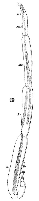 Issued from : W. Giesbrecht in Systematik und Faunistik der Pelagischen Copepoden des Golfes von Neapel und der angrenzenden Meeres-Abschnitte. Fauna Flora Golf. Neapel, 1892, 19 , Atlas von 54 Tafeln. [Taf.10, Fig.19]. Male: 19, P5 (anterior view). Pd = right leg; Ps = left leg.
|
 issued from : N. Phukham in Species diversity of calanoid copepods in Thai waters, Andaman Sea (Master of Science, Univ. Bangkok). 2008. [p.209, Fig.83]. Female (from W Malay Peninsula): a-b, habitus (dorsal and lateral, respectively); c, urosome; d, P5; e, basipod 2 (= Basis) of left P3. Body length after drawing: F = 1.144 mm.
|
 issued from : Mulyadi in Published by Res. Center Biol., Indonesia Inst. Sci. Bogor, 2004. [p.182, Fig.103]. As Clausocalanus arcuicornis major. Male (from 07°29'S, 121°05'E): a, habitus (dorsal); b, P2; c, basis of P2; d, P3; e, basis of P3; f, P5.
|
 Issued from F. Alvarez-Marques in Rev. Fac. Cienc. Univ. Oviedo (Ser. Biologia), (1979-80), 20-21, 1981. [p.161, Pl. I, Figs.6-19]. Female (from Gijon, NW Spain): 6, urosome with spermatophore (lateral); 7, genital segment and spermzatheca (lateral); 8, P5; 9, P5 (with anomaly).
|
 Issued from : O. Tanaka in Spec. Publs. Seto mar. biol. Lab., 10, 1960 [Pl. X, 2, 3]. Female (Indian Ocean): 2, forehead (last thoracic segment and genital segment (lateral); 3, forehead (lateral).
|
 Issued from : O. Tanaka in japanese J. Zool., 1937, VII, 13. [p.252, Fig.2, b, d]. Female (from coast of Heda, Japan): b, Basis of P2 (small specimen); d, P5 (small specimen).
|
 Issued from : O. Tanaka in Publ. Seto Mar. Biol. Lab., 1956, V (3). [p.383, Fig.11, a]. Female (from Izu region, Middle Japan): a, P5 (forma minor).
|
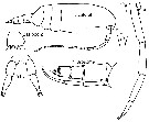
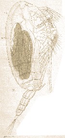 Issued from : E. Chatton in Arch. Zool. Exp. & Gen., 1920, 59, [Pl. IV, 36]. Clausocalanus arcuicornis female (from Banyuls), wich distended stomach by three individuals of Blastodinium pruvoti (Dinoflagellate) t.d.: gut; Bl. P.: Blastodinium pruvoti.
|
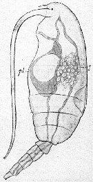 Issued from : E. Chatton in Arch. Zool. Exp. & Gen., 1920, 59, [p.307, Fig.135 bis]. Syndinium sp. (Dinoflagellate) into Clausocalanus arcuicornis female from Banyuls). pl: young plasmode ventrally, with cavity. z: gut zygomens cells of copepod's host.
|
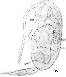
 Issued from : E. Chatton in Arch. Zool. Exp. & Gen., 1920, 59, [p.192, Fig.98]. Clausocalanus arcuicornis female (from Banyuls) patasited by Blastodinium contortum (Dinoflagellate) colourness into the copepod's gut.
|
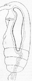
 Issued from : E. Chatton in Arch. Zool. Exp. & Gen., 1920, 59, [Pl. XII]. Clausocalanus arcuicornis with general cavity invaed by a massive plamod of Syndinium carumlac.: lacuna; synd.: plasmod; td.: gut.
|
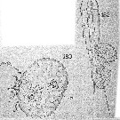 Issued from : E. Chatton in Arch. Zool. Exp. & Gen., 1920, 59, [Pl. XVI, Figs.182, 183]. 182: Clausocalanus arcuicornis juvenil showing two mass of Atelodinium microsporum (Dinoflagellate) plasmods ejected by copepod's anus. 183: one of the two mass enlarged showing small dactyliform-like pseudopods at the surface traducing the amiboid activity of the plasmod.
| | | | | Ref. compl.: | | | Cleve, 1904 a (part., p.188); Pearson, 1906 (p.9, Rem.); Carl, 1907 (p.16); Chatton, 1920 (p.17, parasited): Rose, 1925 (p.152); Gurney, 1927 (p.150)Hardy & Gunther, 1935 (1936) (p.147, Rem.); Massuti Alzamora, 1942 (p.88, Rem.); Wilson, 1942 a (part., p.178); Oliveira, 1945 (p.191); C.B. Wilson, 1950 (part., p.190); Duran, 1955 (p.52); Kott, 1957 (p.6); Yamazi, 1958 (p.148, Rem.); ? Ganapati & Shanthakumari, 1962 (part., p.7, 15); Cervigon, 1962 (p.181, tables: abundance distribution); Gaudy, 1962 (p.93, Rem.: p.104); Grice & Hart, 1962 (p.287, table 3); Duran, 1963 (p.14, Rem.); V.N. Greze, 1963 a (part., tabl.2); Shmeleva, 1963 (part., p.141); ? Grice, 1963 a (p.495); ? Gaudy, 1963 (p.21); Mazza, 1964 (p.293, weight); Unterüberbacher, 1964 (part., p.19, Rem.); Pavlova, 1964 (p.1710); De Decker, 1964 (part., p.15, 20, 30); De Decker & Mombeck, 1964 (?part., p.12); ? Anraku & Azeta, 1965 (p.13, Table 2, fish predator); Grice & Hulsemann, 1965 (? part., p.223); ? Shmeleva, 1965 b (p.1350, lengths-volume -weight relation); Mazza, 1966 (part., p.70); Pavlova, 1966 (part., p.43); Deevey, 1966 (part., p.155, Rem., Table 3), Grice & Hulsemann, 1967 (? part., p.14); Fleminger, 1967 a (tabl.1); Ehrhardt, 1967 (p.738, geographic distribution, Rem.); De Decker, 1968 (?part., p.45); Evans, 1968 (p.12); Delalo, 1968 (? part., p.137); Harder, 1968 (p156, Table 1, behaviour vs. density discontinuity); Berdugo & Kimor, 1968 (p.447); Champalbert, 1969 a (? part., p.629); Morris, 1970 (p.2300); El-Maghraby Dowidar, 1970 (p.81); Dowidar & El-Maghraby, 1970 (p.267); Park, 1970 (p.475); Itoh, 1970 (tab.1); Timonin, 1971 (p.281, trophic group);Deevey, 1971 (p.224); Gamulin, 1971 (p.381, tab.2); Salah, 1971 (p.319); Rudyakov, 1972 (p.886, Table 1: sinking rate); Razouls S., 1972 b (p.2, respiration); Apostolopoulou, 1972 (p.327, 341, fig.2); Gaudy, 1972 (p.175, 231, figs. 33-35, annual cycle); Della Croce & al., 1972 (p.1, fig.2, Rem.); Bainbridge, 1972 (p.61, Appendix Table I: vertical distribution vs day/night, Table II: %, Table IV); Björnberg, 1973 (p.312, 385); Fleminger & Hulsemann, 1973 (p.340, chart); Chatton & M.O. Soyer, 1973 (p.27, Rem.: p.33, parasite); P. Nival & S. Nival, 1973 (p.135, mouth parts, grazing); Desgouille, 1973 (p.1, 131, Rem.: p.138); Corral Estrada & Pereiro Muñoz, 1974 (tab.I); S. Razouls, 1974 (147, oxygen rate); de Bovée, 1974 (p.109, 124); Peterson & Miller, 1975 (p.642, 650, Table 3, interannual abundance); 1976 (p.14, Table 1, 2, 3, abundance vs interannual variations); 1977 (p.717, Table 1, seasonal occurrence); Carter, 1977 (1978) (p.35); Deevey & Brooks, 1977 (p.256, tab.2, Station "S"); Fernandez, 1978 (p.97, metabolism/food, Rem.: Table 19); Comaschi Scaramuzza, 1978 (p.17); Porumb, 1980 (p.168); Herman & Mitchell, 1981 (p.739, Table 1, 2, 3, length-volume); Herman & Sameoto, 1981 (p.228, Table 1, 2, abundance); Kovalev & Schmeleva, 1982 (p.83); Vives, 1982 (p.290); Rudyakov, 1982 (p.208, Table 2); Smith S.L., 1982 (p.1331, abundance, monsoon effect); Castel & Courties, 1982 (p.417, Table II, spatial distribution); Greze & al., 1983 (p.17, Rem.: p.24); Turner & Dagg, 1983 (p.16); Tremblay & Anderson, 1984 (p.6: Rem.); Guangshan & Honglin, 1984 (p.118, tab.); Scotto di Carlo & al., 1984 (p.1041); Mayzaud O. & al., 1984 (p.15, feeding/enzyme); Binet, 1984 (tab.3); Sameoto, 1984 (p.767, vertical migration); Longhurst, 1985 (tab.2); Regner, 1985 (p.11, Rem.;:p.27); Brenning, 1985 a (p.28, Table 2); Moraitou-Apostolopoulou, 1985 (p.303, occurrence/abundance in E Mediterranean Sea); Jansa, 1985 (p.108, Tabl.V); Gaudy, 1985 (p.279, Tab.3); Madhupratap & Haridas, 1986 (p.105, tab.1); Renon, 1987 (tab.2); Comaschi Scaramuzza, 1987 (tab.1); Lozano Soldevilla & al., 1988 (p.58); Jimenez-Perez & Lara-Lara, 1988; Wiebe al., 1988 (tab.7); Herman, 1989 (p.247); Suarez & al., 1990 (tab.2); Ianora & al., 1990 (p.249, fig., parsitism effects); Madhupratap & Haridas, 1990 (p.305, fig.5: vertical distribution night/day; fig.7: cluster); Hirakawa & al., 1990 (tab.3); Scotto di Carlo & al., 1991 (p.271); Hattori, 1991 (tab.1, Appendix); Shih & Marhue, 1991 (tab.2, 3); Yoo, 1991 (tab.1); Suarez & Gasca, 1991 (tab.2); Hirakawa, 1991 (p.376: fig.2); Suarez, 1992 (App.1); Seguin & al., 1993 (p.23, Table 2: abundance, %); Landry & al., 1994 (p.55, abundance, grazing); Landry & al., 1994 a (p.73, grazing, gut evacuation); Verheye & al., 1994 (p.155); Palomares Garcia & Vera, 1995 (tab.1); Hirakawa & al., 1995 (tab.2); Shih & Young, 1995 (p.72); Webber & Roff, 1995 (tab.1); Kotani & al., 1996 (tab.2); Go & al., 1997 (tab.1); Suarez-Morales & Gasca, 1997 (p.1525); Park & Choi, 1997 (Appendix); Padmavati & al., 1998 (p.349); Hsieh & Chiu, 1998 (tab.2); Mauchline, 1998 (tab.24, 30, 58, 64); Noda & al., 1998 (p.55, Table 3, occurrence); Suarez-Morales, 1998 (p.345, Table 1); Suarez-Morales & Gasca, 1998 a (p109); Seridji & Hafferssas, 2000 (tab.1); Dolganova & al., 1999 (p.13, tab.1); Lavaniegos & Gonzalez-Navarro, 1999 (p.239, Appx.1); Onishchik, 1999 (p.76); Bragina, 1999 (p.195); Fernandez-Alamo & al., 2000 (p.1139, Appendix); El-Sherif & Aboul Ezz, 2000 (p.61, Table 3: occurrence); Suarez-Morales & Gasca, 2000 (1247, tab.1); Pinchuk & Paul, 2000 (p.4, table 1, % occurrence); ; Lopez-Salgado & al., 2000 (tab.1); Moraitou-Apostolopoulou & al., 2000 (tab.I); Madhupratap & al., 2001 (p. 1345, vertical distribution vs. O2, figs.4, 5: clusters, Rem.: p.1353); Holmes, 2001 (p.42); Fragopoulu & al., 2001 (p.49, tab.1); El-Serehy & al., 2001 (p.116, Table 1: abundance vs transect in Suez Canal); Sameoto & al., 2002 (p.12); Peterson & al. 2002 (p.381, Table 2, interannual abundance); Zerouali & Melhaoui, 2002 (p.91, Tableau I); Keister & Peterson, 2003 (p.341, Table 1, abundance, cluster species vs hydrological events); Gaudy & al., 2003 (p.357, tab.1); Vukanic, 2003 (139, tab.1); Vieira & al., 2003 (p.S163, Table 2, abundance); Hwang & al., 2003 (p.193, tab.2); Hsiao & al., 2004 (p.325, tab.1); Hsieh & al. 2004 (p.397, tab. 1, p.399, tab.2); Rezai & al., 2004 (p.489, tab.2, p.495, tab.8); Daly Yahia & al., 2004 (p.366, fig.4, tab.1); Lan & al., 2004 (p.332, tab.1); Lo & al.*, 2004 (p.218, tab.1, fig.6); Lo & al., 2004 (p.89, tab.1); Peralba & Mazzocchi, 2004 (p.645, figs. 3, 6); Fernandez de Puelles & al., 2004 (p.654, fig.7); Vukanic & Vukanic, 2004 (p.9, tab. 2, 3); Kazmi, 2004 (p.229); Obuid Allah & al., 2005 (p.123, occurrence % vs metal contamination); Licandro & al., 2005 (p.153); Queiroga & al., 2005 (p.195, table 1); Zuo & al., 2006 (p.159, tab.1, abundance, fig.8: stations group); Isari & al., 2006 (p.241, tab.II); Marques & al., 2006 (p.297, tab.III); Hwang & al., 2006 (p.943, tabl. I); Dias & Araujo, 2006 (p.38, Rem., chart); Zervoudaki & al., 2006 (p.149, Table I); Hooff & Peterson 2006 (p.2610); Durbin & Casas, 2006 (p.2537, Table 2a, 2b); Hwang & al., 2007 (p.24); Fernandez de Puelles & al., 2007 (p.338, fig.7); Valdés & al., 2007 (p.103: tab.1); Busatto, 2007 (p.26, Tab.3); S.C. Marques & al., 2007 (p.213, fig.6); Marques S.C. & al., 2007 (p.725, Table 1, fig.4, climate variability); Dur & al., 2007 (p.197, Table IV); Zakaria, 2007 (p.238, Table 2, spatial distribution); Khelifi-Touhami & al., 2007 (p.327, Table 1); Jitlang & al., 2008 (p.65, Table 1); McKinnon & al., 2008 (p.844 : Tab.I, p.848: Tab. IV); Cabal & al., 2008 (289, Table 1); Humphrey, 2008 (p.83: Appendix A); Lan Y.C. & al., 2008 (p.61, Table 1, % vs stations); Tseng L.-C. & al., 2008 (p.153, Table 2, occurrence vs geographic distribution); Morales-Ramirez & Suarez-Morales, 2008 (p.519); Lopez Ibarra, 2008 (p.1, Table 1, 2, fig.11: abundance); Fernandes, 2008 (p.465, Tabl.2); Rossi, 2008 (p.90: Tableau XII); Ayon & al., 2008 (p.238, Table 4: Peruvian samples); Pagano, 2009 (p.116); C.-Y. Lee & al., 2009 (p.151, Tab.2); Peterson, 2009 (p.73, Rem.: p 78); Galbraith, 2009 (pers. comm.); Skovgaard & Salomonsen, 2009 (p.425, Table 2); Zhang W & al., 2009 (p.261, table 2); Chiba & al., 2009 (p.1846, Table 1, occurrence vs temperature change); Lan Y.-C. & al., 2009 (p.1, Table 2, % vs hydrogaphic conditions); Primo & al., 2009 (p.341, Table1, interannual variations); C.E. Morales & al., 2010 (p.158, Table 1); Brugnano & al., 2010 (p.312, Table 2, 3, fig.8); Hafferssas & Seridji, 2010 (p.353, Table 2, 3); Hafferssas & al., 2010 (p.1281, Table III, abundance vs spatial distribution); Hernandez-Trujillo & al., 2010 (p.913, Table 2); Dias & al., 2010 (p.230, Table 1); Cornils & al., 2010 (p.2076, Table 3); Schnack-Schiel & al., 2010 (p.2064, Table 2: E Atlantic subtropical/tropical, Fig.4, 6, 7, Tabe 4); Hidalgo & al., 2010 (p.2089, fig.4, Table 2, cluster analysis); Sun & al., 2010 (p.1006, Table 2); Mazzocchi & Di Capua, 2010 (p.425); Medellin-Mora & Navas S., 2010 (p.265, Tab. 2); Hsiao S.H. & al., 2011 (p.475, Appendix I); Maiphae & Sa-ardrit, 2011 (p.641, Table 2); Pillai H.U.K. & al., 2011 (p.239, Table 3, vertical distribution); Moscatello & al., 2011 (p.80, Table 4); Selifonova, 2011 a (p.77, Table 1, alien species in Black Sea); S.C. Marques & al., 2011 (p.59, Table 1, seasonal variability); Tutasi & al., 2011 (p.791, Table 2, abundance distribution vs La Niña event); Kâ & Hwang, 2011 (p.155, Table 3: occurrence %); Mazzocchi & al., 2011 (p.1163, Table II, fig.6, long-term time-series 1984-2006); Isari & al., 2011 (p.51, Table 2, abundance vs distribution); Chen H; & al., 2011 (p.84, spatial & temporal variations); Tseng L.-C. & al., 2011 (p.47, Table 2, occurrences vs mesh sizes); Andersen N.G. & al., 2011 (p.71, Fig.3: abundance); Keister & al., 2011 (p.2498, interannual variation); Salah S. & al., 2012 (p.155, Tableau 1); Shiganova & al., 2012 (p.61, Table 4); Uysal & Shmeleva, 2012 (p.909, Table I); Miloslavic & al., 2012 (p.165, Table 2, transect distribution); Brugnano & al., 2012 (p.207, Table 3); DiBacco & al., 2012 (p.483, Table S1, ballast water transport); Krsinic & Grbec, 2012 (p.57, 61: abundance); Tseng & al., 2012 (p.621, Table 3: abundance); Mazzocchi & al., 2012 (p.135, annual abundance 1984-2006); Gonçalves & al., 2012 (p.321, abundance vs climatic variability); Jang M.-C & al., 2012 (p.37, abundance and seasonal distribution); Lavaniegos & al., 2012 (p. 11, Appendix); Dorgham & al., 2012 (p.473, Table 3: abundance %); Hidalgo & al., 2012 (p.134, Table 2, 3, figs.5, 6, abundance vs coastal upwelling); Takahashi M. & al., 2012 (p.393, Table 2, water type index); Belmonte & al., 2013 (p.222, Table 2, abundance vs stations); in CalCOFI regional list (MDO, Nov. 2013; M. Ohman, comm. pers.); Palomares-Garcia & al., 2013 (p.1009, Table I, abundance vs environmental factors); Tachibana & al., 2013 (p.545, Table 1, seasonal change 2006-2008); Tseng & al., 2013 (p.507, seasonal abundance); Tseng & al., 2013 a (p.1, Table 3, 4, abundance); Jagadeesan & al., 2013 (p.27, Table 3, 4, 5, 6, fig.11, seasonal abundance); Anjusha & al., 2013 (p.40, Table 3, abundance & feeding behavior); Peijnenburg & Goetze, 2013 (p.2765, genetic data); Lidvanov & al., 2013 (p.290, Table 2, % composition); Terbiyik Kurt & Polat, 2013 (p.1163, Table 2, seasonal distribution); Hwang & al., 2014 (p.43, Appendix A: seasonal abundance); Fernandez de Puelles & al., 2014 (p.82, Table 3, seasonal abundance); Ortega & al., 2014 (p.495, Table I); Bonecker & a., 2014 (p.445, Table II: frequency, horizontal & vertical distributions); Lopez-Ibarra & al., 2014 (p.453, fig.6, Table 2, biogeographical affinity); Pansera & al., 2014 (p.221, Table 2, abundance); Zaafa & al., 2014 (p.67, Table I, occurrence); Mazzocchi & al., 2014 (p.64, Table 3, 4, 5, spatial & seasonal composition %); Pino-Pinuer & al., 2014 (p.83, Table 1, fig.3, abundance variation vs time); Fierro Gonzalvez, 2014 (p.1, Tab. 3, 5, occurrence, abundance); Zakaria, 2014 (p.3, Table 1, abundance vs 1960-2000); Dias & al., 2015 (p.483, Table 2, abundance, biomass, production); Zakaria & al., 2016 (p.1, Table 1, 3, 4); Benedetti & al., 2016 (p.159, Table I, fig.1, functional characters); Ortega & al., 2017 (p.123, fig.1, 6, table 2, abundance, %) ; Marques-Rojas & Zoppi de Roa, 2017 (p.495, Table 1); El Arraj & al., 2017 (p.272, table 1, 2); Benedetti & al., 2018 (p.1, Fig.2: ecological functional group); Belmonte, 2018 (p.273, Table I: Italian zones); Chaouadi & Hafferssas, 2018 (p.913, Table II: occurrence); Abo-Taleb & Gharib, 2018 (p.139, Table 5, occurrence %); Palomares-Garcia & al., 2018 (p.178, fig.3: relative frequency, Table 1); Hirai & al., 2020 (p.1, Fig. 5: cluster analysis (OTU), spatial distribution). | | | | NZ: | 20 | | |
|
Carte de distribution de Clausocalanus arcuicornis par zones géographiques
|
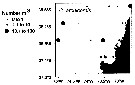
| | | | | | | | | | | | 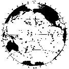 issued from : B. Frost & A. Fleminger in Bull. Scripps Inst. Oceanogr. Univ. California, San Diego, 1968, 12. [p.50, Chart 5, a]. issued from : B. Frost & A. Fleminger in Bull. Scripps Inst. Oceanogr. Univ. California, San Diego, 1968, 12. [p.50, Chart 5, a].
Occurrence of C. arcuicornis in samples examined; closed circles represent samples examined; open circles represent samples in which adults were found; bars through open circles represent samples from which specimens were removed for measurements. |
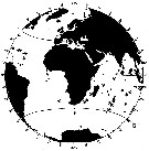 issued from : B. Frost & A. Fleminger in Bull. Scripps Inst. Oceanogr. Univ. California, San Diego, 1968, 12. [p.51, Chart 5, b]. issued from : B. Frost & A. Fleminger in Bull. Scripps Inst. Oceanogr. Univ. California, San Diego, 1968, 12. [p.51, Chart 5, b].
Occurrence of C. arcuicornis in samples examined; closed circles represent samples examined; open circles represent samples in which adults were found; bars through open circles represent samples from which specimens were removed for measurements. |
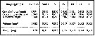 issued from : A.A. Shmeleva in Bull. Inst. Oceanogr., Monaco, 1965, 65 (n°1351). [Table 6:13 ]. Clausocalanus arcuicornis (from South Adriatic). issued from : A.A. Shmeleva in Bull. Inst. Oceanogr., Monaco, 1965, 65 (n°1351). [Table 6:13 ]. Clausocalanus arcuicornis (from South Adriatic).
Dimensions, volume and Weight wet. Means for 50-60 specimens. Volume and weight calculated by geometrical method. Assumed that the specific gravity of the Copepod body is equal to 1, then the volume will correspond to the weight. |
 issued from : C. de O. Dias & A.V. Araujo in Atlas Zoopl. reg. central da Zona Econ. exclus. brasileira, S.L. Costa Bonecker (Edit), 2006, Série Livros 21. [p.38]. issued from : C. de O. Dias & A.V. Araujo in Atlas Zoopl. reg. central da Zona Econ. exclus. brasileira, S.L. Costa Bonecker (Edit), 2006, Série Livros 21. [p.38].
Chart of occurrence in Brazilian waters (sampling between 22°-23° S). |
 issued from : R. Gaudy in Tethys, 1972, 4 (1). [p.237, Fig.36]. issued from : R. Gaudy in Tethys, 1972, 4 (1). [p.237, Fig.36].
Schematic quantitative abundance of Clausocalanus arcuicornis in the Gulf of Marseille (Mediterranean Sea) established from samples during the period between April 1962 to December 1967.
Nota: Gaudy (p.233) points to 5 generations per year. |
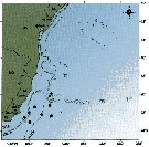
 Issued from : P. Hidalgo, R. Escribano, M. Fuentes, E. Jorquera & O. Vergara in Progr. Oceanogr., 2012, 92-98. [p.140, Fig.5. Spatial distribution of a dominant copepod species (ind m3) found off central-southern Chile in summer 2009. Abundance are mean values in the upper 0-200 m layer. Issued from : P. Hidalgo, R. Escribano, M. Fuentes, E. Jorquera & O. Vergara in Progr. Oceanogr., 2012, 92-98. [p.140, Fig.5. Spatial distribution of a dominant copepod species (ind m3) found off central-southern Chile in summer 2009. Abundance are mean values in the upper 0-200 m layer.
Nota: The upwelling region of central-southern Chile is located at mid latitudes within the eastern boundary upwelling region of Chile and Peru. |
 Issued from S. Razouls in XXIII rd Congress of Athens, 3-11 November 1972. [p.2]. Oxygen consumed by individual (adult) in the Banyuls Bay and equivalent carbon asked. Issued from S. Razouls in XXIII rd Congress of Athens, 3-11 November 1972. [p.2]. Oxygen consumed by individual (adult) in the Banyuls Bay and equivalent carbon asked.
(1) Hydrological season in the stability period: Eté = Summer: 18-20 °C; Hiver = Winter: 13-10°C.
Espèces = species; Saison = Season; Lg céph.= cephalothoracic length; an = individual. |
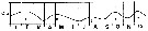
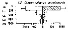 Issued from : M. Madhupratap & P. Haridas in J. Plankton Res., 12 (2). [p.312, Fig.5]. Issued from : M. Madhupratap & P. Haridas in J. Plankton Res., 12 (2). [p.312, Fig.5].
Vertical distribution of calanoid copepod (mean +1 SE), abundance No/100 m3. 42- Clausocalanus arcuicornis.
Night: shaded, day: unshaded.
Samples collected from 6 stations located off Cochin (India), SE Arabian Sea, November 1983, with a Multiple Closing Plankton Net (mesh aperture 300 µm), in vertical hauls at 4 depth intervalls (0-200, 200-400, 400-600, 600-1000 m). |
| | | | Loc: | | | Cosmopolite (tropical & temperate): Benguela Current, South Africa (E & W), Namibia, G. of Guinea, off Lagos, Dakar, off S Cape Verde Is., Morocco-Mauritania, Cap Ghir (Morocco), Canary Is., off Madeira, Portugal, Gijon, Bay of Biscay, off Rio de La Plata (shelfbreak: in Acha & al., 2020), Brazil (S, Campos Basin, Vitoria-Cabo de Sao Tomé), Caribbean Colombia, Venezuela, Bahia de Mochima, Cariaco Basin, Caribbean Sea, Venezuela, Jamaica, Yucatan, Gulf of Mexico, Florida, Sargasso Sea, off Bermuda: Station "S" (32°10'N, 64°30'W), Long Island, Georges bank, Gulf Stream (41°N, 58°W), off SE Nova Scotia, off SE Newfoundland, Ireland, Portugal, Mondego estuary, Ibero-moroccan Bay, off W Tangier, Medit. (Alboran Sea, Habibas Is., Sidi fredj coast, Castellon, Baleares, Algiers, Gulf of Annaba, El Kala shelf, off Barcelona, Banyuls, Marseille, Toulon Harbour, Genova, Ligurian Sea, Lake Faro, Napoli, Tyrrhenian Sea, Strait of Messina, Taranto, Malta, Adriatic Sea, Vlora Bay, Venezzia, Ionian Sea, Aegean Sea, Thracian Sea, Iskenderun Bay, Lebanon Basin, W Egyptian coast, Alexandria, Black Sea), Suez Canal, Hurghada, Safâga, off Sharm El-Sheikh, Red Sea, G. of Aden, Arabian Sea, Natal, Madagascar, Rodrigues Is., Indian, G. of Mannar, Palk Bay, Bay of Bengal, Barren Island, W Malay Peninsula (Andaman Sea), Australie (North West Cape), Straits of Malacca, Flores Sea, Ambon Bay, SW Celebes, China Seas (Yellow Sea, East China Sea, South China Sea), Taiwan Strait, Taiwan (E, SW, W, NW, N, Mienhua Canyon, NE), Okinawa, S Korea, Japan Sea, Tsushima Straits, Korea Strait, Nagazaki, Japan, Kuchinoerabu Is., Tokyo Bay, Kuroshio zone, off Sanriku, S Okhotsk Sea, Kamchatka, Pacif. (equatorial - temperate), Vancouver Is., off Wasington coast, Oregon (Yaquina, off Newport), California, Santa Monica Basin, Baja California (Bahia Magdalena, W), G. of California, La Paz, G. of Tehuantepec, Guaymas Basin, Clipperton Is., Costa Rica (Dome), off W Guatemala, W Costa Rica, W Pacif. (equatorial), SE Australia, ? Great Barrier, New Caledonia, New Zealand, Tasmania, S Pacif. (NPFZ), Galapagos-Ecuador, Peru, Chile (S, off Valparaiso, Concepcion, off Santiago).
Neotype: adult female from 32°06.4' S, 179°57' E. | | | | N: | 288 ? | | | | Lg.: | | | (14) F: 1,55-1,16; M: 1,25-1,22; (30) F: 1,62-1,15; M: 1,17-0,97; (55) F:1,18-1,29; (128) F: 1,13-1,16; (131) F: 1,62-1,15; M: 1,17-0,97; (290) F: 1,15-1,5; M: 0,9-1,15; (374) F: 1,245-1,1; M: 1,15-0,975; (920) F: 1,26; (991) F: 1,08-1,62; M: 0,97-1,2; (1122) M: 1,15; (1138) F: 1,54-1,08; M: 1,02-0,90; {F: 1,08-1,62; M: 0,90-1,25}
The mean female size is 1.294 mm (n = 19; SD = 0.2052), and the mean male size is 1.078 mm (n = 15; SD = 0.1223). The size ratio (male : female) is 0.82 (n = 6; SD = 0.0745). | | | | Rem.: | épipélagique.
Certaines localisations nécessitent confirmation avant 1969, voire même après cette date par méconnaissance du travail de Frost & Fleminger (1968), d'où un nombre de citations discutables indiquées ci-dessus, as for example in the Suez Bay and in the Canal by Gurney, 1927, p.150, without figure and text).
Voir aussi les remarques en anglais | | | Dernière mise à jour : 28/10/2022 | |
|
|
 Toute utilisation de ce site pour une publication sera mentionnée avec la référence suivante : Toute utilisation de ce site pour une publication sera mentionnée avec la référence suivante :
Razouls C., Desreumaux N., Kouwenberg J. et de Bovée F., 2005-2024. - Biodiversité des Copépodes planctoniques marins (morphologie, répartition géographique et données biologiques). Sorbonne Université, CNRS. Disponible sur http://copepodes.obs-banyuls.fr [Accédé le 17 avril 2024] © copyright 2005-2024 Sorbonne Université, CNRS
|
|
|
|


;)
;)
;)
;)
;)
;)
;)
;)
;)
;)
;)
;)
;)
;)
;)
;)
;)
;)
;)
;)
;)
;)
;)
;)
;)
;)
;)
;)
;)
;)
;)

;)
;)
;)
;)