|
|
 |
|
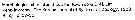
Cyclopoida ( Order ) |
|
|
|
Oithonidae ( Family ) |
|
|
|
Oithona ( Genus ) |
|
|
| |
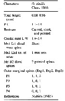
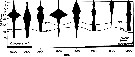
Oithona similis-Group Claus, 1866 (F,M) | |
| | | | | | | Syn.: | ? Oithona helgolandica Claus, 1863 (p.105, fig.M);
O. spinifrons Boeck, 1864; Brady, 1878 (p.90); Thompson & Scott, 1903 (p.255);
Oithona helgolandica : Sars, 1900 (p.119); Pearson, 1906 (p.32); Sars, 1913 (1918) (p.8, Rem.: p. 207, figs.F,M); T. Scott, 1914 (p.8, fig.F); Pesta, 1920 (p.551); Campbell, 1929 (p.322, Rem.); Rose, 1929 (p.56); 1933 a (p.281, figs.F,M); Massuti Alzamora, 1942 (p.102, Rem.); Lysholm & al., 1945 (p.42); Davis, 1949 (p.73, figs.F,M); Fleury, 1950 (p.47, fig.2); Hansen K.V., 1951 (p.231, migration vs. discontinuity layer); Gundersen, 1953 (p.1, 26, seasonal abundance); Crisafi, 1959 b (p.49, figs.F,M, Rem.); Gaudy, 1962 (p.93, 99, Rem.: p.116) ; Duran, 1963 (p.25); Giron-Reguer, 1963 (p.56); Gaudy, 1963 (p.30, Rem.); Shmeleva, 1963 (p.141); Vilela, 1965 (p.12); Mazza, 1966 (p.73); 1967 (p.363, 377, fig.70, p.401, fig.76); Séguin, 1968 (p.488); Vinogradov, 1968 (1970) (p.268); Ramirez, 1969 (p.87, fig.F, Rem.); Champalbert, 1969 a (p.641); Della Croce & al., 1972 (p.1, fig.2, Rem.); Razouls, 1972 (p.95, Annexe: p.105, figs.F,M); Valentin, 1972 (p.349, fig.9: seasonal abundance); Desgouille, 1973 (p.1, 131, Rem.: p.136, fig.16); Vives & al., 1975 (p.53, tab.II, III, IV); Gaudy, 1976 (p.77, fig.1, 6, Table I, II, III, production); Davis C.C., 1976 (p.37, fig.2, reproductive characteristics); Falconetti & Seguin, 1977 (p.188); Vaissière & Séguin, 1980 (p.23, tab.2); Castel & Courties, 1982 (p.417, Table II, fig.4, spatial & monthly distribution); Vives, 1982 (p.295); Patriti & al., 1984 (tab.1); Scotto di Carlo & al., 1984 (p.1041); Regner, 1985 (p.11, Rem.: p.40); Jansa, 1985 (p.108, Tabl.I, II, III, IV, V); Lozano Soldevilla & al., 1988 (p.61); Pancucci-Papadopoulou & al., 1990 (p.199); Valdes & al., 1990 (tab.2); Kouwenberg & Razouls, 1990 (p.23, climatic change); Huys & Boxshall, 1991 (p.358, 360, 442, 465); Villate, 1991 a (fig.4); Santos & Ramirez, 1991 (p. 82, 83); Jouffre & al., 1991 (p.489, lagoon); Seguin & al., 1993 (p.23, Table 2: abundance, %); Santos & Ramirez, 1995 (p.133, Tabl. I, fig.2, 3); Fernandez de Puelles & al., 1996 (p.97, occurrence: p.101); Seridji & Hafferssas, 2000 (tab.1); Holmes & Gotto, 2000 (p.3, Rem.); Sautour & al., 2000 (p.531, Table II, abundance); d'Elbée, 2001 (tabl.1); Zerouali & Melhaoui, 2002 (p.91, Tableau I, fig.5); Gaudy & al., 2003 (p.357, tab.1); Vukanic, 2003 (p.139, tab.1); Daly Yahia & al., 2004 (p.366, fig.1, tab.1); Marrari & al., 2004 (p.667, tab.1); Vukanic & Vukanic, 2004 (p.361, tab. 1, fig.1); Rawlinson & al., 2005 (p.205, tidal exchange); Uriarte & Villate, 2005 (p.863, tab.I); Marques & al., 2006 (p.297, tab.III); Khelifi-Touhami & al., 2007 (p.327, Table 1); Cabal & al., 2008 (289, Table 1); Licandro & Icardi, 2009 (p.17, Table 4); Hafferssas & Seridji, 2010 (p.353, Table 2); Drira & al., 2010 (p.145, Tanl.2); Antacli & al., 2010 (p.71, Table 1, 2, Figs.4, 6); Rekik & al., 2012 (p.336, Table 1, abundance); Sabatini & al., 2012 (p. 33, Table 3, abundance vs stations transect); Spinelli & al., 2012 (p.39, potential prey for fish); Sobrinho-Gonçalves & al., 2013 (p.713, Table 2, fig.8, seasonal abundance vs environmental conditions); Zaafa & al., 2014 (p.67, Table I, occurrence); Antacli & al., 2014 (p.17, occurrence vs community structure).
Oithona spp (mainly similis : Atkinson & Shreeve, 1995 (p.1291, vertical distribution, grazing); Atkinson, 1996 (p.85, Table 3, 5, fig.1, feeding); Atkinson & Sinclair, 2000 (p.46, zonal distribution)
Oithona similis aff. helgolandica : Acha & al., 2020 (p.1, Table 3: occurrence % vs ecoregions, Table 5: indicator ecoregions).
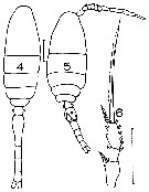
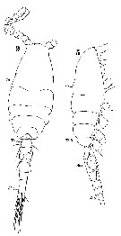
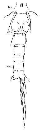
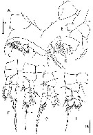
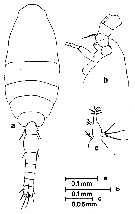
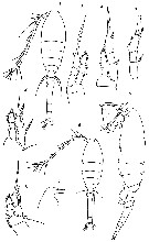
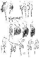
Oithona spp. (miscellaneous species): Roff & al., 1995 (p.165, naupllii vs. bacteriophagy/picoplankton, naupliar production); | | | | Ref.: | | | Claus, 1866 (p.14); Giesbrecht, 1892 (p.537, 548, figs.F,M); Wheeler, 1901 (p.186, figs.F,M, Rem.); Giesbrecht, 1902 (p.28: Rem.Thompson & Scott, 1903 (p.236, 255); Farran, 1908 b (p.88); Wolfenden, 1911 (p.363); Lysholm, 1913 (p.7); Rosendorn, 1917 a (p.24, figs.F,M); Sars, 1918 (p.207, figs.F,M, Rem.); Willey, 1920 a (p.22, Rem.); Lysholm & Nordgaard, 1921 (p.28); Mori, 1929 (p.199, fig.F); Kiefer, 1929 g (p.7, Rem.F,M); Farran, 1929 (p.210, 283); Rose, 1929 (p.55); Wilson, 1932 a (p.314, figs.F,M); Jespersen, 1934 (p.125, fig.33); Farran, 1936 a (p.124); Mori, 1937 (1964) (p.112, figs.F,M); Dakin & Colefax, 1940 (p.116, fig.F); Jespersen, 1940 (p.90); Vervoort, 1951 (p.148, Rem.); Lindberg, 1955 a (p.464: Rem.); Shen & Bai, 1956 (p.226, figs.F,M); Vervoort, 1957 (p.146, Rem.); Crisafi, 1959 b (p.53 & suiv., Rem.); Tanaka, 1960 (p.62, figs.F,M); Kasturirangan, 1963 (p.75, 76, figs.F,M); Tanaka, 1964 (p.13); Marques, 1966 (p.11); Faber, 1966 (p.191, figs.N); Pallares, 1968 b (p.31, figs.F,M); Wellershaus, 1970 (p.483, 484); Minoda, 1971 (p.44); Shih & al., 1971 (p.55, 155, 214); Bossanyi & Bull, 1971 (p.15, Rem.); Bradford, 1971 b (p.28); 1972 (p.48, figs.F,M); Björnberg, 1972 (p.87); Shuvalov, 1972 (1975) (p.172, figs., Rem.); Chen & al., 1974 (p.30, figs.F,M, p.74: Rem., Tab.1); Sullivan & al., 1975 (p.176, figs.Md); Shuvalov, 1976 (in Kos, 1976, Vol. II., figs.F, Rem.); Nishida & al., 1977 (p.149, figs.F,M, Rem.); Shih & Laubitz, 1978 (p.50, 51); Séret, 1979 (p.160, figs.F); Dawson & Knatz, 1980 (p.9, figs.F,M); Shuvalov, 1980 (p.115, figs.N,F,M, Rem.M); Björnberg & al., 1981 (p.663, figs.F); Schnack, 1982 (p.89, figs.: Mx2, Md, Mxp); Gardner & Szabo, 1982 (p.108, figs.F,M); Nishida, 1985 a (p.88, figs.F, Rem.F, p.129); Sazhina, 1985 (p.91, figs. Nauplius); Zheng Zhong & al.,1984 (1989) (p.261, figs.F,M); Nishida, 1986 (p.386); Yoo & Lim, 1993 (p.91, 96, 97, Table 1); Kim & al., 1993 (p.271); Mazzocchi & al., 1995 (p.219, figs.F, Rem.); Menshenina & Melnikov, 1995 (p.128); Chihara & Murano, 1997 (p.939, Pl.194, 200: F,M); Schnack-Schiel & al., 1998 (p.173); Bradford-Grieve & al., 1999 (p.886, 966, figs.F); Conway & al., 2003 (p.204, figs.F,M, Rem.); Conway, 2006 (p.22, copepodides 1-6, Rem.); Ferrari & Dahms, 2007 (p.35, Rem. N, p. 60, 65, copepodites); Avancini & al., 2006 (p.126, Pl. 94, figs.F, Rem.); Vives & Shmeleva, 2010 (p.76, figs.F,M, Rem.); Cheng F. & al., 2013 (p.119, molecular biology, GenBank); Jose & al., 2014 (p.31, Tabl.1, 2, figs.); Cornils & Wend-Heckmann, 2015 (p.243, Table 1, fig. 2: molecular biology); Cepeda & al., 2016 (p.1, Table I: worldwide variation, fig.1: former selected drawings O. similis/O. helgolandica); Cornils & al., 2017 (p.473, species complex | 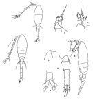 Female: 1, 1', habitus (dorsal view); 2, 2' P1; 3, Head, (lateral); issued from : Tanaka, 1960. 4, Furca; issued from : Nishida, 1985. Male: 5, habitus (lateral); issued from : Tanaka, 1960. 6, Urosome (dorsal); issued from Nishida, Tanaka & Omori in Bull. Plankton Soc. Jap., 1977, 24 (2): 119-158.
|
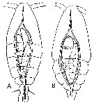
 issued from : M.G. Mazzocchi, G. Zagami, A. Ianora, L. Guglielmo, N. Crescenti & J. Hure in Atlas of Marine Zooplankton Straits of Magellan. Copepods; L. Guglielmo & A. Ianora (Eds.), 1995. [p.220, Fig.3.40.1]. Female: A, habitus (dorsal view); B, idem (lateral view); C, rostrum (lateral view); D, P1; E, P2; F, P3; G, P4. Nota: Prosome 1.2 times urosome. Proportional lengths of urosomites and furca 15:36:14:12:12:11 = 100
|
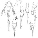
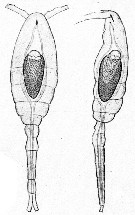
 issued from : G.O. Sars in An Account of the Crustacea of Norway. Vol. VI. Copepoda Cyclopoida. Published by the Bergen Museum, 1913 (1918). [Pl. III]. As Oithona helgolandica. Female & Male (from Norway).
|
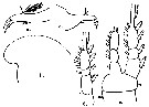
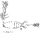
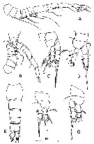
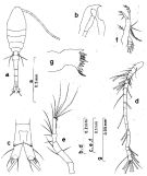 Issued from : S. Nishida in Bull. Ocean Res. Inst., Univ. Tokyo, 1985, No 20. [p.89, Fig.50]. Female: a, habitus (dorsal); b, forehead (lateral); c, anal segment and caudal rami (dorsal); d, A1; e, A2; f, Md (mandibular palp); g, Md (biting edge). Nota: Proportional lengths of urosome segments and caudal ramus 13:34:15:14:14:11. A1 with posteroventral row of minute teeth on segments 2-22.
|
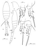
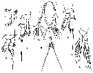
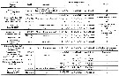
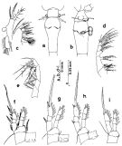 Issued from : S. Nishida in Bull. Ocean Res. Inst., Univ. Tokyo, 1985, No 20. [p.90, Fig.51]. Female: a, thoracic segment 5 and genital segment (dorsal); b, idem (lateral right side); c, Mx1; d, Mx2; e, Mxp; f, P1; g, P2; h, P3; i, P4. Nota after Vives & Shmeleva (2010, p.76): Setal formula on outer margin (in first) and inner margin (in second) of exopod segments (from proximal to distal) of P1 to P4: P1: 1, 1, 2; 0, 1, 4. P2: 1, 0, 1; 0, 1, 5 P3: 1, 0, 1; 0, 1, 5. P4: 0, 0, 1; 0, 1, 5. Male: after Vives & Shmeleva (2010, p.76): Setal formula on outer margin (in first) and inner margin (in second) of exopod segments (from proximal to distal) of P1 to P4: P1: 1, 1, 2; 0, 1, 4. P2: 1, 1, 2; 0, 1, 5 P3: 1, 1, 2; 0, 1, 5. P4: 1, 1, 2; 0, 1, 5.
|
 issued from : Q.-c Chen & S.-z. Zhang & C.-s. Zhu in Studia Marina Sinica, 1974, 9. [Pl.1, Figs.1-7]. Female (from China Seas): 1, habitus (dorsal); 2, forehead (lateral); 3, P2; 4, P3; 5, P4. Nota: According to Breemen (1908) and Shen & Bai (1956), the exopod 3 of P4 is not provided with a single spine, our specimens are provided with an outer spine on the same segment, agreeing well with Tanaka's (1960) description. Male: 6, habitus (dorsal); 7, P3.
|
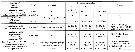
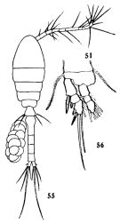 issued from : C.-j. Shen & S.-o. Bai in Acta Zool. sin., 1956, 8 (2). [Pl.VII, Figs.55-56]. Female (from Chefoo); 55, habitus (dorsal); 56, P1. Nota: The armatures of the endopods are similar in both sexes, but those of the exopods are different in some points (See infra Table)
|
 issued from : C.-j. Shen & S.-o. Bai in Acta Zool. sin., 1956, 8 (2). [p.226]. Table: Armature of P1 to P4.
|
 issued from : J.M. Bradford in Mem. N. Z. Oceonogr. Inst., 1972, 54. [p.51, Fig.14, (4-6]. Female (from Kaikoura, New Zealand): 4, habitus (dorsal); 6, exopod of P2. Male: 5, habitus (dorsal). Scale bars: 0.1 mm (4, 5, 6). Nota: One of the most common copepods in the Kaikoura plankton.
|
 issued from : I. Rosendorn in Wiss. Ergebn. dt. Tiefsee-Exped. \\\"Valdiviella\\\", 1917, 23. [p.25, Fig.13]. Female: a, Md (mandibular palp). Nota: Proportion of lengths (p.cent) Prosome : 56.41, Urosome : 43.59 . Relative lengths of urosomal segments and caudal rami: 5: 12: 5: 4: 5: 3.5. Setal formula of the exopod swimming legs P1 to P4 (Se = outer setae ; Si = inner setae), P1 : 1, 1, 2 Se ; 0, 1, 5 Si ; P2 : 1, 0, 1 Se ; 0, 1, 5 Si ; P3 : 1, 0, 1 Se ; 0, 1, 5 Si ; P4 : 0, 0, 1 Se ; 0, 1, 5 Si . Male: b, forehead (lateral); c, Md (mandibular palp); d, P2; e, P3. Nota: Proportion of total lengths (p.cent) Prosome : 64.18, Urosome : 35.82 . Relative lengths of urosomal segments and caudal rami: 7 : 17 : 9 : 8.5 : 6.5 : 7: 7. Setal formula of the exopod swimming legs P1 to P4 (Se = outer setae ; Si = inner setae), P1 : 1, 1, 2 Se ; 0, 1, 5 Si ; P2 : 1, 1, 2 Se ; 0, 1, 5 Si ; P3 : 1, 1, 2 Se ; 0, 1, 5 Si ; P4 : 1, 1, 2 Se ; 0, 1, 5 Si .
|
 issued from : T. Mori in Zool. Mag. Tokyo, 1929, 41 (486-487). [Pl. VII, Fig.19]. Female (from Chosen Strait, Korea-Japan): 19, habitus (dorsal).
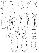
|
 issued from : T. Mori in The Pelagic copepoda from the neighbouring waters of Japan, 1937 (1964). [Pl. 62, Figs.1-6]. Female: 1, Md; 2, P1; 3, P2; 4, habitus (dorsal); 5, P3; 6, P4.
|
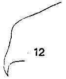 issued from : T. Mori in The Pelagic copepoda from the neighbouring waters of Japan, 1937 (1964). [Pl. 62, Fig.12]. Female: 12, forehead (lateral).
|
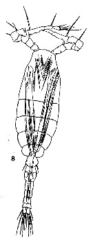 issued from : T. Mori in The Pelagic copepoda from the neighbouring waters of Japan, 1937 (1964). [Pl. 62, Fig.8]. Male: 8, habitus (dorsal).
|
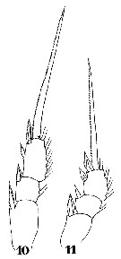
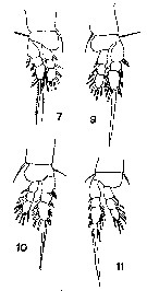 issued from : T. Mori in The Pelagic copepoda from the neighbouring waters of Japan, 1937 (1964). [Pl. 62, Figs.7, 9, 10, 11]. Male: 7, P1; 9, P2; 10, P3; 11, P4.
|
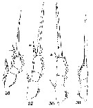
 issued from : V.S. Shuvalov in Opred. Faune SSSR, Nauka, Leningrad, 1980, 125. [p.117, Fig.25]. Female: 1, habitus (dorsal); 2, prosome (dorsal); 3-4, forehead (lateral); 5, same (dorsal); 6, P1; 7, P2 (basipod , exopod); 8, P3; 9, urosome (dorsal); 10-13, anal segment and caudal rami; 14-16, prosome (dorsal). Nota: 10, 11: from Atlantic Ocean; 12 from Arctic Ocean; 13: from Yellow Sea; 14: from Arctic Ocean; 15-16: from Atlantic ocean.
|
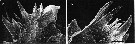
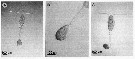 issued from : A. Skovgaard & N. Daugbjerg in Protist, 2008, 159. [p.403, Fig.1 A-C]. Living Paradinium spp.-infected copepods from the NW Mediterranean Sea. A: P. poucheti (PaOi21) gonosphere attaced to the urosome of its host, Oithona similis. B: same at higher magnification. C: P. poucheti (PaOi01) gonosphere attached to the urosome of the copepod O. similis.
|
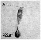 issued from : A. Skovgaard & N. Daugbjerg in Protist, 2008, 159. [p.403, Fig.2 A]. Paradinium poucheti gonosphere attached of its living host O. similis from the Godthabbsfjord, Greenland.
|
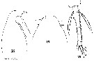
 Issued from : W. Giesbrecht in Systematik und Faunistik der Pelagischen Copepoden des Golfes von Neapel und der angrenzenden Meeres-Abschnitte. Fauna Flora Golf. Neapel, 1892, 19 , Atlas von 54 Tafeln. [Taf.44, Figs.5, 9]. Male: 5, habitus (lateral); 9, habitus (dorsal).
|
 Issued from : W. Giesbrecht in Systematik und Faunistik der Pelagischen Copepoden des Golfes von Neapel und der angrenzenden Meeres-Abschnitte. Fauna Flora Golf. Neapel, 1892, 19 , Atlas von 54 Tafeln. [taf.44, Fig.3]. Male: 3, A2 (over view).
|
 Issued from : W. Giesbrecht in Systematik und Faunistik der Pelagischen Copepoden des Golfes von Neapel und der angrenzenden Meeres-Abschnitte. Fauna Flora Golf. Neapel, 1892, 19 , Atlas von 54 Tafeln. [Taf.44, Fig.8]. Male: 8, urosome (ventral).
|
 Issued from : W. Giesbrecht in Systematik und Faunistik der Pelagischen Copepoden des Golfes von Neapel und der angrenzenden Meeres-Abschnitte. Fauna Flora Golf. Neapel, 1892, 19 , Atlas von 54 Tafeln. [Taf.44, Figs.10, 11]. Male: 10, P2; 11, P1.
|
 Issued from : W. Giesbrecht in Systematik und Faunistik der Pelagischen Copepoden des Golfes von Neapel und der angrenzenden Meeres-Abschnitte. Fauna Flora Golf. Neapel, 1892, 19 , Atlas von 54 Tafeln. [Taf. 34, Figs.18, 19, 21]. Female: 18-19, forehead (lateral and dorsal, respectively); 21, urosome (dorsal).
|
 Issued from : W. Giesbrecht in Systematik und Faunistik der Pelagischen Copepoden des Golfes von Neapel und der angrenzenden Meeres-Abschnitte. Fauna Flora Golf. Neapel, 1892, 19 , Atlas von 54 Tafeln. [Taf. 34, Figs.36-39]. Female: 36, exopodite of P1; 37, exopodite of P2; 38, exopodite of P3; 39, exopodite of P4. Se = outer seta.
|
 issued from : C. Razouls in Th. Doc. Etat Fac. Sc. Paris VI, 1972, Annexe. [Fig.61]. As Oithona helgolandica sensu Sars, 1913 (1918). Female (from Banyuls, G. of Lion): A, forehead (dorsal view); B, Md; C, Mxp; D, Mx2; E, P3; F, P2; G, P4; H, P1. Nota: anomaly on the basispodal segment 1 of P3 with 1 inner seta.
|
 issued from : C. Razouls in Th. Doc. Etat Fac. Sc. Paris VI, 1972, Annexe. [Fig.62]. As Oithona helgolandica. Male: A-B, A1; C, P4; D, P3; E, urosome; F, P1; G, P2. Nota: anomaly on exopodal segment 3 of P1 missing 1 inner seta.
|
 issued from : B.K. Sullivan, C.B. Miller, W.T. Peterson & A.H. Soeldner in Mar. Biol., 1975, 30. [p.181, Fig.6, C-D]. Oithona similis (from 50°N, 145°W) female: C-D, SEM of two Md;.
|
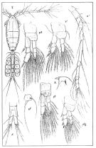
 Issued from : S. Nishida, O. Tanaka & M. Omori in Bull. Plankton Soc. Japan, 1977, 24 (2). [p.150, Fig.21]. Female (from Sagami Bay and adjacent waters): a, habitus (dorsal), b, forehead (lateral); c, Md; d, Mx1; e, P1; f, P2; g, P3; h, P4. Nota: Setae formula of exopod P1 to P4 (outer setae in first, inner setae in second). P1: 1,1,2; 0,1,4. P2: 1,0,1; 0,1,5. P3: 1,0,1; 0,1,5. P4: 0,0,1; 0,1,5. Prosome length/urosome length = 1.21-1.40.
|
 Issued from : S. Nishida, O. Tanaka & M. Omori in Bull. Plankton Soc. Japan, 1977, 24 (2). [p.150, Fig.22]. Female (from Sagami Bay and adjacent waters ): a, habitus (dorsal); b, forehead (lateral); c, Md. Nota: Setae formula of exopod P1 to P4 (outer setae in first, inner setae in second). P1: 1,1,2; 0,1,4. P2: 1,1,2; 0,1,5. P3: 1,1,2; 0,1,5. P4: 1,1,2; 0,1,5. Prosome length/urosome length = 1.73-1.90.
|
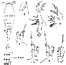
 Issued from : O. Tanaka in Spec. Publs. Seto mar. biol. Lab., 10, 1960 [Pl. XXVII]. Female (from Indian Ocean and Antarctic): 1, habitus (dorsal); 2, P1; 3, exopod of P2; 4, P3; 5, P4; 6, habitus (dorsal; other specimen); 7, forehead (lateral); 8, P1. Nota: Prosome and urosome proportional lengths 55 to 45. Rostrum curved slightly posteriorly, not visible from the dorsal. Urosomal segments and caudal rami in the proportional lengths 10 : 36 : 15 : 15 : 14; 10 = 100 Male (from Cape of Good Hope): habitus (lateral). Nota: Prosome and urosome in the proportional lengths 63 to 37. Urosomal segments and caudal rami in the proportional lengths 12 : 26 : 18 : 12 : 9 : 11 : 12 = 100. The A1 has the knee-joint between the segments 11 and 12. Remarks: The female varied in size from 0.71 to 1.05 mm, but no difference was found among them in general appearence and in the structure of the appendages. Farran (1929) reported that some Antarctic specimens had a rather broad and flattened cephalothorax, but their appendages agreed well with the typical type.
|
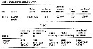
 Issued from : O. Tanaka in Spec. Publs. Seto mar. biol. Lab., 10, 1960 [p. 63]. Female: Proportional lengths of segments of A1.
|
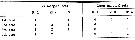
 Issued from : O. Tanaka in Spec. Publs. Seto mar. biol. Lab., 10, 1960 [p. 63]. Female: Number of outer marginal spine and inner marginal seta of the exopodal segment of swimming legs P1 to P4.
|
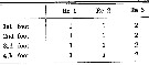
 Issued from : O. Tanaka in Spec. Publs. Seto mar. biol. Lab., 10, 1960 [p. 63]. Female: Number of Inner and outer marginal setae of endopodal segments of the swimming legs P1 to P4.
|
 Issued from : O. Tanaka in Spec. Publs. Seto mar. biol. Lab., 10, 1960 [p. 64]. Male: Number of outer marginal spine on the exopodal segments of swimming legs P1 to P4.
|
 Issued from : J.J. Jose, A. Chandran, L. Alex & A.P. Lipton in Not. Sci. Biol., 2014, 6 (1). [p.33, Tab. 2). Setal formula of the exopod (outer and inner margins) and endopod of the four legs (P1 to P4) of female Oithona similis from SW India (Vizhinjam to Calicut)
|
 Issued from : A. Willey in Rep. Can. arct. Exped., 1920, VII: Crustacea, Part K: Marine Copepoda. [p.23 K]. Oithona similis (from off Bernard Harbour). Relative lengths of the last thoracic segment, the abdominal segments and the furca (= caudal rami).
|
 Issued from : K.-I. Yoo & D.-H. Lim in The Korean J. Syst. Zool., 1993, 9 (2) [p.97: key of female] in Korean Waters: Morphological characters of Oithona similis female :
1 - Anterior part of prosome rounded in dorsal view.
2 - Rostrum pointed ventrally. 3 - Length of A1 longer than that of prosome. 4 - Exopod 2nd segment of P1 with 1 spine. 5 - Exopod 3rd segment of P2 with 1 spine.
|
 Issued from : G.D. Cepeda, M.E. Sabatini, C.L. Scioscia, Ramirez F.C. & M.D. Viñas in ZooKeys, 2016, 552. [p.5, Table I] . Worldwide variation in the key characters commonly reported for the determination of O. similis/helgolandica.
|
 Issued from : G.D. Cepeda, M.E. Sabatini, C.L. Scioscia, Ramirez F.C. & M.D. Viñas in ZooKeys, 2016, 552. [p.6, Table I, continued]. Worldwide variation in the key characters commonly reported for the determination of O. similis/helgolandica.
|
 Issued from : G.D. Cepeda, M.E. Sabatini, C.L. Scioscia, Ramirez F.C. & M.D. Viñas in ZooKeys, 2016, 552. [p.7, Table I, continued]. Worldwide variation in the key characters commonly reported for the determination of O. similis/helgolandica.
|
 Issued from : G.D. Cepeda, M.E. Sabatini, C.L. Scioscia, Ramirez F.C. & M.D. Viñas in ZooKeys, 2016, 552. [p.9, Fig.I]. Former selected drawings of O. similis/helgolandica.
A, B: O. spinifrons Boeck, 1864 (= ? O. helgolandica Claus), female body and ''one of swimming feet'' (= leg 4?) (after Brady, 1878, Plates XIV and XXIV A).
C-F: O. similis exopod of legs I to 4 (after Giesbrecht 1893 [1892] (Plate34).
C_J: O. helgolandica, female body, legs 1-2 and leg 4 (after Sars, 1913, Olate III).
K-O: O. similis, female body and legs I to 4 (after Nishida 1985, fig.50 and 51).
Original illustrations were faithfully copied in all details and arranged to facilitate comparisons. Scale bars only provided in Nishida (1985).
|
 Issued from : E. Chatton in Arch. Zool. Exp. & Gen., 1920, 59, [p.147, Fig.48]. Oithona similis female (from Banyuls) parasited by Blastodinium oviforme (Dinoflagellate), lonely triblastic form from dorsal and lateral views.
|
 Issued from : E. Chatton in Arch. Zool. Exp. & Gen., 1920, 59, [p.129, Fig.33, 34]. Oithona similis female (from Banyuls) parasited by Blastodinium oviforme (Dinoflagellate): A, slender individuals in the copepod's gut ; B, parasite ovoid-like, lonely and monoblasic into the copepod's gut.
|
 Issued from : C. Razouls in Ann. Inst. océanogr., Paris, 1994, 70 (1). [p.184]. Caractéristiques morphologiques de Oithona similis lato sensu, femelle et mâle adultes. Terminologie et abbréviations: voir à Calanus propinquus.
|
 Issued from : A. Cornils & B. Wend-Heckmann in Helgol. Mar. Res., 2015, 69. [p.246, Table 1]. Oithona similis charcteristics in the semi-enclosed bight in the northern Germann Wadden Sea (North Sea) Compare with O. nana, O. plumifera, O. atlantica and O. davisae in the North Sea.
| | | | | Compl. Ref.: | | | Vanhöffen, 1897 a (p.281); Mrazek, 1902 (p.517, 524); Cleve, 1904 a (p.193); Pearson, 1906 (p.32); Damas & Koefoed, 1907 (p.395, tab.II); Sars, 1909 b (p.39); Chatton, 1920 (p.17, parasites); Rose, 1925 (p.152); Wilson, 1932 (p.49); Hardy & Gunther, 1935 (1936) (p.189, Rem.); Fish, 1936 b (p.168, biology); Jespersen, 1939 (p.79, Rem., Table 25, 26, 27, 28, 29, 30); Bogorov, 1939 b (p.706); C.B. Wilson, 1942 a (p.196); Sewell, 1948 (p.345, 461, 487, 515); C.B. Wilson, 1950 (p.271); Fleury, 1950 (p.47, fig.2); Østvedt, 1955 (p.15: Table 3, p.17, 77); Yamazi, 1958 (p.153, Rem.); Minoda, 1958 (p.253, Table 1, 2, abundance); Deevey, 1960 (p.5, Table II, annual abundance, Rem.: fig.18, 19); H. Schulz, 1961 (p.57); Fagetti, 1962 (p.39); Grice & Hart, 1962 (p.287, table 4: abundance); Marshall & Orr, 1962 (tab.1, 3); Grice, 1962 a (p.101); Björnberg, 1963 (p.77, Rem.: Juv.); Lacroix & Bergeron, 1963 (p.59, Tableau III); Unterüberbacher, 1964 (p.32); De Decker & Mombeck, 1964 (p.13); Dimov, 1964 b (p.33, Tableau 1); Carter, 1965 (Rem.: p.351); Shmeleva, 1965 b (p.1350, lengths-volume -weight relation); Marshall & Orr, 1966 (p.513, 521, fig. I, 2, Table 1, 3, 4, 5, 6, 7, feeding, respiration); Faber, 1966 a (p.419, 421); Pavlova, 1966 (p.44); Harding, 1966 (p.17, 71); Furuhashi, 1966 a (p.295, vertical distribution vs mixing Oyashio/Kuroshio region); Neto & Paiva, 1966 (p.29, Table III, annual cycle); Mazza, 1967 (p.356: Rem.); Pertsova, 1967 (p.240); Maclellan D.C., 1967 (p.101, 102: occurrence); Hargrave & Geen, 1968 (p.332, phosphorus excretion); Dimov, 1968 (p.506); Greze & al., 1968 (p.1066, annual variation); Zaika, 1968 (p.311, P/B quotient); Kovalev, 1968 a (p.441, fig.1); Vinogradov, 1968 (1970) (p.49, 50, 53, 63, 64, 243); Harder, 1968 (p156, Table 1, behaviour vs. density discontinuity); Salah, 1971 (p.320); Paulmier, 1971 (p.168); Martens, 1972 (p.30, fecal pellets); Björnberg, 1973 (p.357, 359: Rem., 388); Arndt & Heidecke, 1973 (p.599, 603, fig.3); Eriksson, 1973 (p.37, fig.26-29, annual cycle); 1973 b (p.113, 117); Frolander & al., 1973 (p.277, annual cycles); Hirota, 1974 (p.1, Table 3, fig.4, 5); Peterson & Miller, 1975 (p.642, 650, Table 3, interannual abundance); Anraku, 1975 (p.79, microdistribution); Hirota & Hara, 1975 (p.115, fig.5, 6); Kolosova, 1975 (p.92, fig.2, 3, Table 1); Conover & Mayzaud, 1975 (p.151, fig.5, abundance); Peterson & Miller, 1976 (p.14, Table 1, 2, 3, abundance vs interannual variations); Porumb, 1976 (p.91); Grindley, 1977 (p.341, Table 2, fig.2, 3, 4); Hanaoka, 1977 (p.267, 300, abundance); Sameoto, 1977 (p.1); Peterson & Miller, 1977 (p.717, Table 1, seasonal occurrence); McLaren, 1978 (p.1330, 1338: life history); Conover, 1978 (p.66, 69, feeding); Poulet, 1978 (p.1126, grazing); Hernroth, 1978 (p.1, Rem.: p.7); Mayzaud & Poulet, 1978 (p.1144, feeding); Knatz, 1978 (p.68, Table 1, fig.3, abundance, %); Peterson & al., 1979 (p.467, Table 1, Fig.11); Poulet & Marsot, 1980 (p.198, Fig.2, feeding); Kosobokova, 1980 (p.167, seasonal changes, vertical distribution, age composition); Fukuchi & Tanimura, 1981 (p.37); Gagnon & Lacroix, 1981 (p.401, Table 1, tidal effect); Hoshiai & Tanimura, 1981 (p.44); Mackas & Sefton, 1982 (p.1173, Table 1); Uye S-i., 1982 (p.149, relation length-weight-C-N); Buchanan & Sekerak, 1982 (p.41, Table 3: vertical distribution); Citarella, 1982 (p.791, 798: listing, frequency, fig.5, Tableau II, V); Kovalev & Shmeleva, 1982 (p.85); Gagnon & Lacroix, 1982 (p.9, fig.4); 1983 (p.289, Table III, tidal estuary); Huntley & al., 1983 (p.143, Table 2, 3); Maranda & Lacroix, 1983 (p.247, estuary); Nishiyama & Hirano, 1983 (p.159, Table 4: length-weight); Hernroth, 1983 (p.835,, Rem.: p.840); Hassel, 1983 (p. 1, fig.6, abundance, distribution); Turner & Dagg, 1983 (p.8, fig.11, 17, vertical distribution); Tremblay & Anderson, 1984 (p.7, Rem.); Drits & Semenova, 1984 (p.755, feeding); Sameoto, 1984 (p.213, Table 1, fig.9); 1984 a (p.767, vertical migration); Fransz & al., 1984 (p.86); Dussart, 1984 (p.25, 64: occurrence): Pieper & Holliday, 1984 (p.226, Fig.3); De Ladurantaye & al., 1984 (p.21, fig.5, advective processes in fjord); Hopkins, 1985 (p.197, Table 1, gut contents); Kimmerer & McKinnon, 1985 (p.150); Musayeva, 1985 (tab.1); Foster & Battaerd, 1985 (p.213); Kawamura & Hirano, 1985 (p.626, Table 1, horizontal distribution); Sameoto & al., 1986 (p.53); Groendahl & Hernroth, 1986 (tab.1); Kawaguchi & al., 1986 (tab.2); Mackas & Anderson, 1986 (p.115, Table 2); Harding & al., 1986 (p.952, Table 3, diel vertical movements); Mikhailovsky, 1986 (p.83, Table 1, ecological modelling); Zmijewska, 1987 (tab.2a); Ceccherelli & al., 1987 (p.571, fig.5); Hopkins & Torres, 1988 (tab.1); James & Wilkinson, 1988 (p.249, Table 1, 2, biomass, carbon ingestion); McLaren & al., 1989 (p.560, life history, annual production); Kosobokova, 1989 (p.27); Springer & al., 1989 (p.359, Fig.5, 10); Citarella, 1989 (p.123, abundance); Cervantes-Duarte & Hernandez-Trujillo, 1989 (tab.3); Coyle & al., 1990 (p.764); Peterson & al., 1990 (p.259, Table V, feeding); Tucker & Burton, 1990 (p.591, tab.1, fig.5, seasonal, spatial variations); Ohman, 1990 (p.257, fig.); Anderson J.T., 1990 (p.127, Rem.: p.131); Dai & al., 1991 (tab.1); Yoo, 1991 (tab.1); Fransz & al., 1991 (p.7 & suiv.); Eslake & al., 1991 (p.93, Table 2, temporal changes); Conover & Huntley, 1991 (p.1, Table 2, 3, 4, polar seas comparison); Huntley & Lopez, 1992 (p.201, Table A1, egg-adult weight, temperature-dependent production); Kimmerer, 1993 (tab.2); Hwang & Choi, 1993 (tab.3); Jiyalal Ram & Goswami, 1993 (p.129, tab.IV); Freire & al., 1993 (tab.3); Richter, 1994 (tab.4.1a); Vinogradov & al., 1994 (tab.1); Gonzalez & al., 1994 (p.331); Landry & al., 1994 (p.55, abundance, grazing); Godhantaraman, 1994 (tab.6); Myung & al., 1994 (tab.1); Sabatini & Kiørboe, 1994 (p.1329, egg production, growth, development); Hwang & Turner, 1995 (p.207, Table 1, 2, fig. 1, 2, 3: swimming behaviour); Ragosta & al., 1995 (Appendix A); Petryashov & al., 1995 (tab.1); Oliveira Dias, 1995 (p.147); Fransz & Gonzalez, 1995 (p.549, production); Shih & Young, 1995 (p.75); Krause & al., 1995 (p.81, Rem.: p.134); Metz, 1995 (p.190); 1996 (p.22, 87); Knox & al., 1996 (tab.1); Kotani & al., 1996 (tab.2); T.G. Nielsen & Sabatini, 1996 (p.79, abundance); Park & Choi, 1997 (p.225, Appendix); Cordell & al., 1997 (p.7, % change vs 1980-1997); Cordell, 1997 (On line pdf); Fransz & Gonzalez, 1997 (p.395, weight-length, biomass vs. N-S transect); Swadling & al., 1997 (p.39, Table 1, , figs. 6, 7, 8, grazing); Falkenhaug & al., 1997 (p.449, spatio-temporal pattern); Nakamura & Turner, 1997 (p.1275, nutrition, respiration, feeding vs. ciliates); Atkinson, 1998 (p.289, Table 1, biological data); Hure & Krsinic, 1998 (p.80, 103); Elwers & Dahms, 1998 (p.150, 151, fig.1, 2, 3, seasonal abundance); Kosobokova & al., 1998 (tab.2); Suarez-Morales & Gasca, 1998 a (p.112); Sameoto & al., 1998 (p.1, Rem. p.7, spatial distribution); Schnack-Schiel & al., 1998 (p.173, abundance, sea ice); Harvey & al., 1999 (p.1, 49: Appendix 5, in ballast water vessel); Siokou-Frangou, 1999 (p.478); Dolganova & al., 1999 (p.13, tab.1); Goldblatt & al., 1999 (p.2619, Fig.5); Halvorsen & Tande, 1999 (p.279, figs.3, 6); Logerwell & Ohman, 1999 (p.428, tab.1); Voronina & Kolosova, 1999 (p.72); Bragina, 1999 (p.196); Abramova, 1999 (p.161, Table 2); B.W. Hansen & al., 1999 (p.233, seasonal abundance & biomass); Razouls & al., 2000 (p.343, tab. 5, Appendix); Ueda & al., 2000 (tab.1); DFO, 2000 (p.1, Rem.: p.4, fig.2, interannual variations); Pepin & Maillet, 2000 (p.1, Rem.: p.8, table 2, interannual variations); Escribano & Hidalgo, 2000 (p.283, tab.2); Kosobokova & Hirche, 2000 (p.2029, tab.2); Selifonova, 2000 (p.68, tab.1); Svensen & Hiørboe, 2000 (p.1155, prey detection vs. hydromechanical or chemical cues ); Musaeva & Suntsov, 2001 (p.511); Fortier M. & al., 2001 (p.1263, fig.6, 7, diel vertical migration); Van Hove & al., 2001 (p.303); Fransz & Gonzalez, 2001 (p.255, tab.1); Chiba & al., 2001 (p.95, tab.4, 7); Beaumont & al., 2001 (p.55); Hidalgo & Escribano, 2001 (p.159, tab.2); Hidalgo & Escribano, 2001 (p.157, fig.4); Li & al., 2001 (p.894, tab.1); Lischka & al., 2001 (p.186); Hunt & al., 2001 (p.374, tab.1); Beaumont & al., 2001 (p.55); Nielsen & al., 2002 (p.301, egg hatching rate); Cabal & al., 2002 (p.869, Table 1, abundance); Dubischar & al., 2002 (p.3871, abundance); Coyle & Pinchuk, 2002 (p.177, fig.2, 3, 4, Table 4, 5, annual variation); Bressan & Moro, 2002 (tab.2); Beaumont & al., 2002 (p.133, tab.1); Viñas & al., 2002 (p.1031); Auel & Hagen, 2002 (p.1013, tab.2, 3); Nielsen & al., 2002 (p.301); Greenwood & al., 2002 (p.17, Table 2); Ringuette & al., 2002 (p.5081, Table 1, Fig.7, population dynamic); Sameoto & al., 2002 (p.13); Peterson & al., 2002 (p.381, Table 2, interannual abundance); Ward & al., 2003 (p.121, tab.4); Peterson & Keister, 2003 (p.2499, interannual variability); Kosobokova & al., 2003 (p.697, tab.2); Ashjian & al., 2003 (p.1235, figs.); Kovalev, 2003 (p.47); Zagorodnyaya & al., 2003 (p.52); Vieira & al., 2003 (p.S163, Table 2, abundance); Karnovsky & al., 2003 (p.289, Appendix 1, 2 (as Oithona similus), auks relation/copepods); Hsieh & al., 2004 (p.398, tab.1, p.399, tab.2); Rezai & al., 2004 (p.490, tab.2, 3, abundance, Rem., p.495, tab.8); Chang & Fang, 2004 (p.456, tab.1); Shushkina & al., 2004 (p.524, tab.2); Zuenko & Nadtochii, 2004 (p.526, tab.1, fig.8); Gislason & Astthorsson, 2004 (p.472, tab.1); Wang & Zuo, 2004 (p.1, Table 2, dominance, origin); Hunt, 2004 (p.1, 43, 47, 74, Table 3.2, 4.4, fig.4.7, 4.11, Rem.: p.97, 100, fig.5.10: seasonal abundance); Vargas & Gonzalez, 2004 (p.151); Lo & al., 2004 (p.89, tab.1); Mackas & al., 2004 (p.875, Table 2); Eiane & Ohman, 2004 (p.183, stage-specific mortality); Hansen F.C. & al., 2004 (p.659, spatio-temporal distribution); Dmoch & Walczowski, 2005 (p.102 + poster); Dias & Bonecker, 2005 (p.100 + poster); Fuentes & Schanck-Schiel, 2005 (p.253); Mazzocchi & al., 2005 (p.155); Manning & Bucklin, 2005 (p.233, Table 1), fig.5); Lischka & Hagen, 2005 (p.910, life history); Bielecka & Zmijewska, 2005 (p.96); Choi & al., 2005 (p.710: Tab.III); Zamon & Welch, 2005 (p.133, fig.5); Calbet & al., 2005 (p.1195, tab.3); Castellani & al., 2005 (p.129, respiration rates vs temperature); Berasategui & al., 2005 (p.485, tab.1); Coyle, 2005 (p.77, tab.2,5); Hopcroft & al., 2005 (p.198, table 2); Mackas & al., 2005 (p.1011, tab.2, 3); Castellani & al., 2005 (p.173, feeding vs. egg production); Reigstad & al., 2005 (p.265, coprophagy); Berasategui & al., 2006 (p.485: fig.2); Zuo & al., 2006 (p.159, tab.1, 3, fig.9, spatial abundance, fig.8: stations group); Ware & McQueen, 2006 (p.28, Table B1, weight ranges); Blachowiak-Samolyk & al., 2006 (p.101, tab.1); Isari & al., 2006 (p.241, tab.II); Hunt & Hosie, 2006 (p.1182, seasonal succession, indicator); 2006 a (p.1203, tab.2, fig.8); Hwang & al., 2006 (p.943, tabl. I) ; Lopez-Ibarra & Palomares-Garcia, 2006 (p.63, Tabl. 1, seasonal abundance vs El-Niño, Rem.: p.70, ); Sterza & Fernades, 2006 (p.95, Table 1, occurence); Dias & Araujo, 2006 (p.73, Rem., chart); Zervoudaki & al., 2006 (p.149, Table I); Hop & al., 2006 (p.182, Table 4, 5: inter-annual variability, fig.14); Willis & al., 2006 (p.39, Table 2, advection vs changes in community structure); Tsujimoto & al., 2006 (p.140, Table1); Escribano, 2006 (p.20, Table 1); Hooff & Peterson, 2006 (p.2610); Papastephanou & al., 2006 (p.3078, Table 3); Deibel & Daly; 2007 (p.271, Table 1, 2, 3, 4, 6b, Rem.: Arctic polynyas); Kattner & al., 2007 (p.1628, Table 1); Albaina & Irigoien, 2007 (p.435: Tab.1); Elliott & Kaufmann, 2007 (p.418); Castellani & al., 2007 (p.1051); Schulz J. & al., 2007 (p.47, vertical zonation analysis); Fielding & al., 2007 (p.2106, tab.1); Walkusz & al., 2007 (p.43); Guglielmo & al., 2007 (p.747, Table 4, 5); Busatto, 2007 (p.26, Tab.2); Valdés & al., 2007 (p.104: tab.1); Biancalana & al., 2007 (p.83, Tab.2, 3); Blachowiak-Samolyk & al., 2007 (p.2716, Table 2); Lischka & Hagen, 2007 (p.443, lipids vs. diet); Lischka & al., 2007 (p.1331, digestive enzyme vs. seasonal); Iversen & Poulsen, 2007 (p.79, coprophagy, clearance, ingestion, coprorhexy); McKinnon & al., 2008 (p.843: Tab.1, p.848: Tab. IV); Isinibilir & al., 2008 (p.745: Tab.1, as similes); Lane & al., 2008 (p.97, fig.11, Tab.6); Ward & al., 2008 (p.241, Appendix II ); Ayon & al., 2008 (p.238, Table 4: Peruvian samples); Walkusz & al., 2008 (p.1, Table 3, abundance); Hirst & Ward, 2008 (p.169, mortality rate); Humphrey, 2008 (p.84: Appendix A); Morales-Ramirez & Suarez-Morales, 2008 (p.522); Coyle & al., 2008 (p.1775, Table 3, 5, fig.11, abundance); Blachowiak-Samolyk & al., 2008 (p.2210, Table 2, 3, 5, fig.4, biomass, composition vs climatic regimes); Tanimura & al., 2008 (p.561, vertical distribution, diel changes); Lopez Ibarra, 2008 (p.1, Table 1, 2, figs.11, 15: abundance); Fernandes, 2008 (p.465, Tabl.2); Selifonova & al., 2008 (p.305, Tabl. 2); Schnack-Schiel & al., 2008 (p.1056, Table 1, 4); Tseng L.-C. & al., 2008 (p.153, fig.5, Table 2, occurrence vs geographic distribution, indicator species); Lan Y.-C. & al., 2008 (p.61, Table 1, % vs stations); Ohtsuka & al., 2008 (p.115, Table 4, 5, in Japan Harbors); Raybaud & al., 2008 (p.1765, Table A1); Skovgaard & Daugbjerg, 2008 (p.401, fig.1 A-C, 2 A, parasited by Paradinium); Darnis & al., 2008, (p.994, Table1, fig.8, 9); Rossi, 2008 (p.90: Tableau XII); Perumal & al., 2008 (p.149, abundance vs hydrographic parameters); Chiba & al., 2009 (p.1846, Table 1, occurrence vs. temperature change); Hopcroft & al., 2009 (p.9, Table 3, Fig.22); Pagano, 2009 (p.116); Peterson, 2009 (p.73, Rem.: p 78); Galbraith, 2009 (pers. comm.); Skovgaard & Salomonsen, 2009 (p.425, Table 2); Telesh & al., 2009 (p.18: Table 2.1); Lan & al., 2009 (p.1, Table 2); Escribano & al., 2009 (p.1083, Table 1, figs.6, 10); Zervoudaki & al., 2009 (p.1475, fig.2); DFO, 2009 (p.1, fig. 13, seasonal variability); Kosobokova & Hirche, 2009 (p.265, Table 4, biomass); Dvoretsky & Dvoretsky, 2009 (p.259, morphological variability vs. zones); 2009 a (p.11, Table 2, abundance); 2009 c (p.165, morphological variations); 2009 d (p.133, egg production vs. zonation); 2009 b (p.1433, life cycle); Narcy & al., 2009 (p.233, seasonal variability of lipid reserves); C.E. Morales & al., 2010 (p.158, Table 1); Hwang J.-S. & al., 2010 (p.220, Table 2, fig.3, 4, %, abundance); Vogedes & al., 2010 (p.1471, lipid sac area vs lipid content); Lidvanov & al., 2010 (p.356, Table 3); Takahashi & al., 2010 (p.317, Table 3, 4, figs.4, 5, 6, 7, 8); Drira & al., 2010 (p.145, Tanl.2); Drif & al., 2010 (p.159, abundance, Rem.: egg production); Pinkerton & al., 2010 (p.469, Fig.13); Hernandez-Trujillo & al., 2010 (p.913, Table 2); Hidalgo & al., 2010 (p.2089, fig.2, 4, Table 2, cluster analysis); Sun & al., 2010 (p.1006, Table 2); Hopcroft & al., 2010 (p.27, Table 1, 2); Dias & al., 2010 (p.230, Table 1, fig.7 a); Mazzocchi & Di Capua, 2010 (p.428); W.-B. Chang & al., 2010 (p.735, Table 2, abundance); Bucklin & al., 2010 (p.40, Table 1, Biol mol.); Kosobokova & Hopcroft, 2010 (p.96, Table 1, fig.7); Bucklin & al., 2010 (p.40, Table 1, Biol mol.); Swadling & al., 2010 (p.887, Table 2, 3, A1, fig.6, abundance, indicator species); Kosobokova & Hopcroft, 2010 (p.96, Table 1, fig.7); Dvoretsky & Dvoretsky, 2010 (p.991, Table 2); 2011 a (p.1231, Table 2; abundance, biomass); Kosobokova & al., 2011 (p.29, Table 2, figs.4, 7, Rem.: Arctic Basins); Hirche & Kosobokova, 2011 (p.2359, Table 3, abundance, biomass %); Pomerleau & al., 2011 (p.1779, Table III, IV); Hsiao S.H. & al., 2011 (p.475, Appendix I); Maiphae & Sa-ardrit, 2011 (p.641, Table 2); Swadling & al., 2011 (p.118, Rem.: p.124); Magris & al., 2011 (p.260, abundance, interannual variability); Tseng L.-C. & al., 2011 (p.47, Table 2, occurrences vs. mesh sizes); Dvoretsky & Dvoretsky, 2011 (p.123, mortality rates vs. salinity); 2011 b (p.469, Table A, abundance, biomass); Yang & al., 2011 a (p.921, Table 2, inter-annual variation 1999-2006); Turner & al., 2011 (p.1066, Table II, abundance 1998-2008); Isari & al., 2011 (p.51, Table 2, abundance vs. distribution); Arendt, 2011 (p.1, Rem. p.23); Mazzocchi & al., 2011 (p.1163, Table I, II, long-term time-series 1984-2006); Pepin & al., 2011 (p.273, Table 2, seasonal abundance); Forest & al., 2011 (p.11418); 2012 (p.1301, figs.7, 8); Zervoudaki & al., 2011 (p.45, fig.3, abundance: Turkish Straits); Takahashi & al., 2011 (p.134, distribution); Beltrao & al., 2011 (p.47, Table 1, density vs. time); Pond & Ward, 2011 (p.105, diatoms role); Ward & al., 2012 (p.78, Table A1, B1, abundance, weight); Cepeda & al., 2012 (p.1, figs.1, 3, Table 1, Molecular systematic); Van Ginderdeuren & al., 2012 (p.3, Table 1); Postel, 2012 (p.327, Table 1, Fig.6); Shiganova & al., 2012 (p.61, fig.3, 4, 5); Glushko & Lidvanov, 2012 (p.138, Tableau 1); Uysal & Shmeleva, 2012 (p.909, Table I); Thompson G.A. & al., 2012 (p.127, Table 2, 3, 5, fig.4, 5, Rem.); DiBacco & al., 2012 (p.483, Table S1, ballast water transport); Jose & al., 2012 (p.20, fig.3 a,b,c: % vs. monsoon); Zizah & al., 2012 (p.79, Table I, Rem.: p.86, 89 as O. helgolandica); Rekik & al., 2012 (p.336, Table 1, abundance); Thompson G. & al., 2012 (p.367, fig.2, 3, Table 3, abundance vs mesh selectivity); Johan & al., 2012 (2013) (p.1, Table 1); Mazzocchi & al., 2012 (p.135, annual abundance 1984-2006); Zamora-Terol & Saiz, 2013 (p.376, Rem.: Table 3, egg production); Sigurdardottir, 2012 (p.1, Table 2.3); Aubry & al., 2012 (p.125, table 1, 3, fig. 6, 8a, b, interannual variation); Miloslavic & al., 2012 (p.165, Table 2, transect distribution); Schulz J. & al., 2012 (p.3, abundance vs. hydrography); Johnson C & al., 2012 (p.1, 15, fig. 23a, 23b, 24a, 24b, seasonal variability, interannual variarions); Stefanova & al., 2012 (p.403, Table 2, interannual abundance); Volkov, 2012 (p.474, Table 6, fig. 6, 11, abundance, distribution, interannual variation); Dvoretsky & Dvoretsky, 2012 (p.1321, Table 2, 3, 4, 5, abundance, biomass, production); Jean & al., 2012 (p.12, Table 3, protein vs environmental metal stress); Salah S. & al., 2012 (p.155, Tableau 1); Krsinic & Grbec, 2012 (p.57, 62: abundance); Huo & al., 2012 (p.1, Table 1: dominance); Demontigny & al., 2012 (p.221, Table II, fig.5, abundance, prey by ichthyoplankton); Dvoretsky V.G., 2012 (p.63, mortality rates vs environmental data); Bode & al., 2012 (p.108, spatial distribution vs time-series, % biomass); Tarling & al., 2012 (p.222, Table 3, seasonal biomass); Aguirre & al., 2012 (p.341, Table I: abundance vs season, figs.4, 67); Lee J. & al., 2012 (p.95, Table 2: abundance, annual & seasonal distribution); Jang M.-C. & al., 2012 (p.37, abundance and seasonal distribution); Hidalgo & al., 2012 (p.134, Table 2, 3, fig.5, 6: spatial distribution) ; Gusmao & al., 2013 (p.279, Table 3, 4, fig.1, sex-specific predation by fish, fig.4: seasonal variation of sex ratio); Gubanova & al., 2013 (in press, p.4, Table 2); Li C. &al., 2013 (p.101, feeding); Belmonte & al., 2013 (p.222, Table 2, abundance vs stations); in CalCOFI regional list (MDO, Nov. 2013; M. Ohman, comm. pers.); Tachibana & al., 2013 (p.545, Table 1, seasonal change 2006-2008); Questel & al., 2013 (p.23, Table 3, interannual abundance & biomass, 2008-2010); Varadharajan & Soundarapandian, 2013 (p.2: occurrence vs. stations); Siokou & al., 2013 (p.1313, fig.4, 8, biomass, vertical distribution); Ojima & al., 2013 (p.1293, Table 2, 3, 4, fig.3, abundance, Rem.); Jagadeesan & al., 2013 (p.27, Table 3, 5, 6, fig.11, seasonal variation); Zamora-Terol & al., 2013 (p.85, abundance); Anjusha & al., 2013 (p.40, Table 3, abundance & feeding behavior); Lee D.B. & al., 2013 (p.1215, Table 1, 2: abundance, composition); Dvoretsky & Dvoretsky, 2013 (p.203, Rem.: p.211, 212, morphometry); Kwasniewski & al., 2013 (p.83, Table 2, 3, abundance); Lidvanov & al., 2013 (p.290, Table 2, % composition); Terbiyik Kurt & Polat, 2013 (p.1163, Table 2, seasonal distribution); Wend-Heckmann, 2013 (p.1-171, molecular biology); Eisner & al., 2013 (p.87, Table 3: abundance vs water structure); Dvoretsky & Dvoretsky, 2013 a (p.205, Table 2, % abundance); Zamora Terol, 2013 (p.89, egg production, Table 2, 3, 4, fig.4, 5, temporal variation, vertical distribution, length vs. temperature, fecondity, feeding rates vs. diets); Zamora-Terol & Saiz, 2013 (p.376, feeding rates, egg production); Hwang & al., 2014 (p.43, Appendix A: seasonal abundance); Fernandez de Puelles & al., 2014 (p.82, Table 3, seasonal abundance); Ward & al., 2014 (p.305, Table 4, abundance in the ''Discovery'' Investigations in the 1930s); Bonecker & a., 2014 (p.445, Table II: frequency, horizontal & vertical distributions); Lopez-Ibarra & al., 2014 (p.453, fig.6, 8, Table 2, biogeographical affinity); Pansera & al., 2014 (p.221, Table 2, abundance); Mazzocchi & al., 2014 (p.64, Table 3, 4, 5, spatial & seasonal composition %) ; Pino-Pinuer & al., 2014 (p.83, Table 1, fig.3, 4, abundance variation vs time); Fierro Gonzalvez, 2014 (p.1, Tab. 3, 4, 5, occurrence, abundance); Castellani & al., 1915 (p.1, annual variations: 1984 - 2013); Dias & al., 2015 (p.483, Table 2, abundance, biomass, production, Table 4: % vs. season); Rojas-Herrera & al., 2016 (p.40, Table 2: temporal abundance); Smoot & Hopcroft, 2016 (p.1, fig.3, abundance vs water mass); Araujo & al., 2016 (p.1, Table 3, abundance, %) ; Zakaria & al., 2016 (p.1, Table 1, 3, 4); Ben Ltaief & al., 2017 (p.1, Table III, Summer relative abundance); Benedetti & al., 2016 (p.159, Table I, fig.1, functional characters); Hansen B.W. & al., 2017 (p.984, pH effects). Marques-Rojas & Zoppi de Roa, 2017 (p.495, Table 1); Benedetti & al., 2018 (p.1, Fig.2: ecological functional group); Coyle & al., 2014 (p.97, table 10, 11, 12); Castellani & al., 2016 (p.703, abundances: long-term series 1984-2013); Ohtsuka & Nishida, 2017 (p.565, 578, Table 22.1, Fig.: 22.3: outermost station-central station); El Arraj & al., 2017 (p.272, table 1, 2, spatial distribution); Madoui & al., 2017 (p.4467, Rem.); Dias & al., 2018 (p.1, Table 4: % vs. season); Hure M. & al., 2018 (p.1, Table 1: abundance, % composition, Table 2: correlations, Rem.: p.12); Palomares-Garcia & al., 2018 (p.178, Table 1: occurrence); Camatti & al., 2019 (p.1, fig.6, Table 3, 4, 5); Hirai & al., 2020 (p.1, Fig. 5: cluster analysis (OTU), spatial distribution). | | | | NZ: | 25 | | |
|
Distribution map of Oithona similis-Group by geographical zones
|
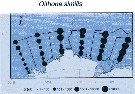
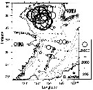
| | | | | | | | | | | | | | | | | | 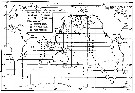 Issued from : S. Nishida in Bull. Ocean Res. Inst., Univ. Tokyo, 1985, No 20. [p.129, Fig.78]. Issued from : S. Nishida in Bull. Ocean Res. Inst., Univ. Tokyo, 1985, No 20. [p.129, Fig.78].
Indo-Pacific geographical distribution of Oithona similis. Dotted line: AC, Arctic Convergence; SC, Subtropical Convergence. |
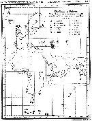 issued from : I. Rosendorn in Wiss. Ergebn. dt. Tiefsee-Exped. "Valdiviella", 1917, 23. [Taf. I]. issued from : I. Rosendorn in Wiss. Ergebn. dt. Tiefsee-Exped. "Valdiviella", 1917, 23. [Taf. I].
The genus Oithona: Distribution of species sampled during the Deutsche Tiefsee Expedition 1898-99.
The size of symbols indicates the relative quantitty of the species. |
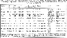
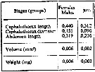 issued from : A.A. Shmeleva in Bull. Inst. Oceanogr., Monaco, 1965, 65 (n°1351). [Table 6: 39]. Oithona similis (from South Adriatic). issued from : A.A. Shmeleva in Bull. Inst. Oceanogr., Monaco, 1965, 65 (n°1351). [Table 6: 39]. Oithona similis (from South Adriatic).
Dimensions, volume and Weight wet. Means for 50-60 specimens. Volume and weight calculated by geometrical method. Assumed that the specific gravity of the Copepod body is equal to 1, then the volume will correspond to the weight. |
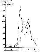
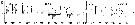
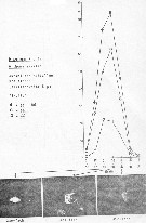
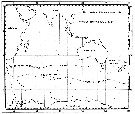
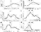
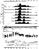 issued from : P.S.B. Digby in J. Mar. Biol. Ass. U.K., 1950, 29. [p.406, Fig.7]. issued from : P.S.B. Digby in J. Mar. Biol. Ass. U.K., 1950, 29. [p.406, Fig.7].
Life history of Oithona similis at station L (5 miles from Plymouth, English Channel).
A: abundance of copepodite stages; B: percentage distribution of stages; C: size-groups of adult females; D: suggested interpretation of generations (or cohorts) succession during the year (1947).
Correlate the size variations with the water temperature at station L4 (p.397, Fig.1).
The author deduces the succession of 5 generations. |
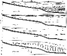
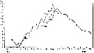 issued from : P.S.B. Digby in J. Mar. Biol. Ass. U.K., 1950, 29. [p.397, Fig.1]. issued from : P.S.B. Digby in J. Mar. Biol. Ass. U.K., 1950, 29. [p.397, Fig.1].
Temperature of the water at 1 and 30 m depth at station L4 (5 miles from Plymouth, English Channel) during 1947. x: surface readings from closer in-shore. |
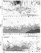
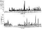
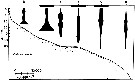 issued from : J.T. Turner & M.J. Dagg in Biol. Oceanogr., 1983, 3 (1). [p.10, Fig.4]. issued from : J.T. Turner & M.J. Dagg in Biol. Oceanogr., 1983, 3 (1). [p.10, Fig.4].
Vertical and inshore-offshore distributions of Oithona similis at pump stations on the Long Island (NW Atlantic) transect (40°31.8'-39°53.2' N, 72°23.6'-72°59.4' W)..
Station numbers are given on the top axis, and dark horizontal bars identify stations sampled at night. |
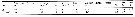
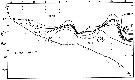 issued from : J.T. Turner & M.J. Dagg in Biol. Oceanogr., 1983, 3 (1). [p.7, Fig.2]. issued from : J.T. Turner & M.J. Dagg in Biol. Oceanogr., 1983, 3 (1). [p.7, Fig.2].
Vertical temperature structure durnig the Long Island transect (40°31.8'-39°53.2' N, 72°23.6'-72°59.4' W; October 1978). |
 issued from : J.T. Turner & M.J. Dagg in Biol. Oceanogr., 1983, 3 (1). [p.24, Fig.11]. issued from : J.T. Turner & M.J. Dagg in Biol. Oceanogr., 1983, 3 (1). [p.24, Fig.11].
vertical distribution of Oithona similis in relation to positions of the 15°C and 10°C water at the time of sampling during the Long Island time series (40°26'N, 72°18'W; October 1978).
Sampling times are given on the bottom axis, and dark horizontal bars identify periods of darkness. |
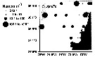
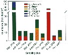
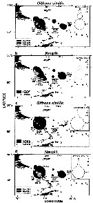 issued from : G.A. Thompson, E. O. Dinofrio & V.A. Alder in Helgol. Mar. Res., 2012, 66. [p.134, Fig.4]. issued from : G.A. Thompson, E. O. Dinofrio & V.A. Alder in Helgol. Mar. Res., 2012, 66. [p.134, Fig.4].
Density and biomass of Oithona similis (a, c) and nauplii (b, d) for summer 2000, 2001 and 2003.
Circle size is proportional to the absolute values of density and biomass.
Zooplankton samples and environmental data were collected at 56 oceanographic stations in Subantarctic and Antarctic waters of the Atlantic sector of the Southern Ocean (the Drake Passage and the Scotia Sea during three austral summers.
Oithona similis, together with small cyclopoids and nauplii, accounted for the largest percentage of the total number of copepods in the community and for the highest biomass value (63 % of total copepod biomass). |
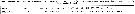
 issued from : J.R. Grindley in Trans. roy. Soc. S. Afr., 42, 3 & 4. [p.353, Fig.4]. issued from : J.R. Grindley in Trans. roy. Soc. S. Afr., 42, 3 & 4. [p.353, Fig.4].
Distribution of Oithona similis from Saldanha Bay to Schrywershoek area (33°S, 18° E).
Compare this distribution with the species in the same site: Pseudodiaptomus hessei, Tortanus capensis, Paracartia longipatella. |
 issued from : S. Eriksson in Zoon, 1976, 4. [p.157, Fig.2]. issued from : S. Eriksson in Zoon, 1976, 4. [p.157, Fig.2].
Seasonal distribution of neritic copepod Oithona similis off Gothenburg (Göteborg), The Skattegatt. (Monthly means for adult specimens during 1968-1973; point : inshore, depth = 10 m; x: offshore, depth > 40 m.
The optimum temperature is 6 to 18°C. range. |
 issued from : S. Eriksson in Zoon, 1976, 4. [p.159, Fig.3, e]. issued from : S. Eriksson in Zoon, 1976, 4. [p.159, Fig.3, e].
Temperature occurrence of neritic copepod Oithona similis off Gothenburg (Göteborg), The Skattegatt.
.Surface salinity of the investigation area varies around 25 p.1000 and the deep water slinity around 34 p.1000. There is a temperature stratification with surface water warmer than 10°C from May to October with maximum of 20°C in August. The coldest period is January to March with surface temperatures of 1-2°C. The deep water ranges between 5 and 10°C.
The hauls were horizontal at 2, 20, and 40 m.
Limits subjectively regarded as the optimum temperature range: 6-18°C. |
 issued from : S. Eriksson in ZOON, 1973, 1. [p.60, Fig.29]. issued from : S. Eriksson in ZOON, 1973, 1. [p.60, Fig.29].
Size distribution of adult females of Calanus helgolandicus (offshore station H6:11°30' N, 57°40'.5 E, The Kattegatt) during 1968-70 in the main series. |
 issued from : S. Eriksson in Mar. Biol., 1974, 26. [p.320, Figs. 2-3] issued from : S. Eriksson in Mar. Biol., 1974, 26. [p.320, Figs. 2-3]
Salinity and temperature curves for main series at offshore station H6 (11°30' N, 57°40'.5 E, The Kattegatt) from March 1968 to November 1970. |
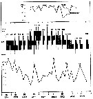
 issued from : I.A. McLaren, M.J. Tremblay, C.J. Corkett & J.C. Roff in Can. J. Fish. Aquat. Sci., 1989, 46. [p.574, Fig.12]. issued from : I.A. McLaren, M.J. Tremblay, C.J. Corkett & J.C. Roff in Can. J. Fish. Aquat. Sci., 1989, 46. [p.574, Fig.12].
Annual cycle of Oithona similis on Emerald Bank (43°30'N, 63°00'W), 1979-80 (upper two panels) and Browns Bank (42°35'N, 65°50'W), 1984-1985 (lower panel).
Successive generations labelled Go, etc. For convenience, Nov. 1979 sample placed at end (after 1980) in uppermost panel, which is abundances as proportions of stages (AD: adults; adult males not distinguished). Middle and lower panels: size-frequencies of adult females as proportions.
The samples were obtained by vertical hauls from near bottom (usually 25 m) by Hensen-type nets (one of 0.250 mm mesh and the other of 0.064 mm mesh) on Emerald Bank and obtained by vertical hauls from near bottom (usually 70-80 m) by Hensen-type nets (one of 0.202 mm mesh and the other of 0.064 mm mesh) on Browns Bank. |
 issued from : I.A. McLaren, M.J. Tremblay, C.J. Corkett & J.C. Roff in Can. J. Fish. Aquat. Sci., 1989, 46. [p.574, Fig.13]. issued from : I.A. McLaren, M.J. Tremblay, C.J. Corkett & J.C. Roff in Can. J. Fish. Aquat. Sci., 1989, 46. [p.574, Fig.13].
Relative frequencies of stages of Oithona similis on Browns Bank (42°35'N, 65°50'W), 1979.
Adult males are clear portion of bar. |
 issued from : P. Martens in M.S. Inst. Meeresk. Christian-Albrechts Univ., 1972. [p.30]. issued from : P. Martens in M.S. Inst. Meeresk. Christian-Albrechts Univ., 1972. [p.30].
Numbers of fecal pellets (n) by width classes (interval from 0.005 mm).
Nota: individuals in culture on Chaetoceros decipiens, C. socialis, Detonula cystifera, Skeletonema costatum and flagellates.
Mean size of fecal pellets: length = 36 ± 8 micrometers; width = 26 ± 5 micrometers. Volume male = 12915 µ3; female = 12387 µ3 |
 issued from : I.A. McLaren inJ. Fish. Res. Board Can., 1978, 35. [p.1339, Fig.8]. issued from : I.A. McLaren inJ. Fish. Res. Board Can., 1978, 35. [p.1339, Fig.8].
Life cycles of Oithona similis in Loch Striven (55°55'N, 05°10'W).
Relative abundance of C V as a percentage of all copepodids (lower panel); size and numbers per haul (including combined hauls from 60 m to 10 m and 10 to 0 m) of adult females (middle panel), and percentage of nauplii and copepodids above 10 m (from split hauls, taken from 60 to 10 m and 10 to 0 m) (upper panel).
Successive generations as infered from peaks in the C V cohorts and size changes designated as Go, G1, etc.
Data from Marshall (1949, tables IX and XVI). |
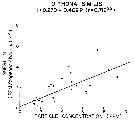 Issued from : R.J. Conover in Rapp. P.-v. Réun. Cons. int. Explor. Mer, 1978, 173. [p.69, Fig.54]. Issued from : R.J. Conover in Rapp. P.-v. Réun. Cons. int. Explor. Mer, 1978, 173. [p.69, Fig.54].
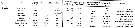
Regression between rate of ingestion (I) for Oithona similis from Bedford Basin, Nova Scotia (Canada) and particle concentration in the same environment. |
 Issued from : M. Anraku in Mar. Biol., 1975, 30. [p.82, Figs. 1, 2]. Issued from : M. Anraku in Mar. Biol., 1975, 30. [p.82, Figs. 1, 2].
Distribution of hydrological factors and abundance of Oithona similis in Oshoro Bay (west Hokkaido, Japan), 30 August 1958, along vertical section from stations 1 to 5 (distance 650 m).
Nota: The plankton samples were collected by means of a plankton pump during the morning hours at the same time as the hydrological observations. Copepodids and adults were counted ans expressed as number of individuals per 20 l.
The distribution of copepods in a limited area seems to be related to the pattern of oceanographic conditions to some extent, but a pattern of contagious distribution is also apparent. See Barnes & Marshall (1951); Cassie (1959); Boyd (1973). |
 Issued from : M. Anraku in Mar. Biol., 1975, 30. [p.84, Fig.5]. Issued from : M. Anraku in Mar. Biol., 1975, 30. [p.84, Fig.5].
Microdistribution of Oithona similis in Oshoro Bay (west Hokkaido, Japan), 28 August 1958, ascertained by pump along vertical section from station 3.
Nota: After the author, it is clear that the results obtained in the present investigations indicate non-random distribution.
The distribution patterns indicated the presence of inhomogeneous distribution with small swarms and irregular layerings.
Large-scale patchiness of plankton has previously been recorded (see Hardy & Gunther, 1935; Rae & Rees, 1947). The results of the present investigation indicate thet the large-scale patch includes small patches of different sizes in both the horizontal and vertical planes.
Simultaneous measurements of certain physical, chemical, and biological parameters (as the the quantitative and qualitative food particles, the occurrence of predators) are necessary to approach an understanding of copepod microdistribution. |
 Issued from : K.M. Swadling, So. Kawaguchi & G.W. Hosie in Deep-Sea Research II, 2010, 57. [p.898, Fig.6 (continued)]. Issued from : K.M. Swadling, So. Kawaguchi & G.W. Hosie in Deep-Sea Research II, 2010, 57. [p.898, Fig.6 (continued)].
Distribution of indicator species Oithona similis from the BROKE-West survey (southwest Indian Ocean) during January-February 2006.
Sampling with a RMT1 net (mesh aperture: 315 µm), oblque tow from the surface to 200 m.
The survey area was located predominantly within the seasonal ice zone, and in the month prior to the survey there was considerable ice coverage over the western section but none over the east.
See map showing sampling sites in Calanus propinquus. |
 Issued from : V.G. Dvoretskii & A.G. Dvoretskii inRussian J. Mar. Biol., 2009, 35 (3). [p.261, Table 2]. Issued from : V.G. Dvoretskii & A.G. Dvoretskii inRussian J. Mar. Biol., 2009, 35 (3). [p.261, Table 2].
Indices of morphological variability of Oithona similis (mean ±error of mean) in the White Sea.
Lc: Cephalothorax length; La: overall length of antennule
Sampled with a Juday net (mesh aperture: 168 µm) in June 2001. 1450 specimens examined in total. |
 Issued from : V.G. Dvoretskii & A.G. Dvoretskii inRussian J. Mar. Biol., 2009, 35 (3). [p.259, Table 1]. Issued from : V.G. Dvoretskii & A.G. Dvoretskii inRussian J. Mar. Biol., 2009, 35 (3). [p.259, Table 1].
Hydrological characteristics of distinguished regions in the White Sea in June 2001. |
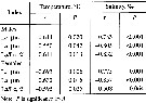 Issued from : V.G. Dvoretskii & A.G. Dvoretskii inRussian J. Mar. Biol., 2009, 35 (3). [p.261, Table 3]. Issued from : V.G. Dvoretskii & A.G. Dvoretskii inRussian J. Mar. Biol., 2009, 35 (3). [p.261, Table 3].
Correlation of morphological characteristics of Oithona similis with hydrological conditions in the White Sea.
Temperature and salinity throughout the water column. Correlation analysis: means compared with Mann-Whitney non-parametric test.
Nota: A tendency toward increasing the antennule length along the axix from cold areas with high salinity toward warmer regions with relatively low salinity is clearly noticeable. This is due to a decrease in water density, where temperature increases and salinity goes down.
The morphological variations have adaptative significance and are determined by environmental factors. |
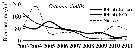 Issued from : A.F. Volkov in Russian Journal of Marine Biology, 2012, 38 (7). [p.483, Fig.6] Issued from : A.F. Volkov in Russian Journal of Marine Biology, 2012, 38 (7). [p.483, Fig.6]
Dynamics in the biomass of Oithona similis in the eastern Bering Sea from 2003-2011 years. |
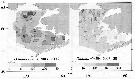 Issued from : A.F. Volkov in Russian Journal of Marine Biology, 2012, 38 (7). [p.490, Fig.11] Issued from : A.F. Volkov in Russian Journal of Marine Biology, 2012, 38 (7). [p.490, Fig.11]
Distribution of Oithona similis in the eastern Bering Sea in the fall. Biomass in mg/m3. |
 Issued from : Jan Schulz & coll. in Progr. Oceanogr., 2012, 107; [p.8, Fig.4 [modified]); Issued from : Jan Schulz & coll. in Progr. Oceanogr., 2012, 107; [p.8, Fig.4 [modified]);
Seasonal patterns in the abundance of Acartia longiremis in the Bornholm Basin (central Baltic Sea) between March 2002 and May 2003. The scaling is normalised to one and vertical lines indicate sampling dates.
Sampling performed in stacked, 10m intervals from a few meters above the seafloor to the surface with a multinet (Hydro-bios, Kiel, 50 µm mesh size) on nine focus stations.
Compare with annual cycle in Acartia longiremis, Acartia bifilosa, Centropages hamatus, Temora longicornis and other forms. |
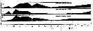
 Issued from : Jan Schulz & coll. in Progr. Oceanogr., 2012, 107; [p.6, Fig.2]. Issued from : Jan Schulz & coll. in Progr. Oceanogr., 2012, 107; [p.6, Fig.2].
Vertical profiles of temperature, salinity and oxygen in the central Bornholm Basin (Baltic Sea) at position 55.3016° N, 15.7966° E. |
 Issued from : C. Séret in Thesis 3ème Cycle, UPMC, Paris 6. 1979, Annexe. [p.53]. Issued from : C. Séret in Thesis 3ème Cycle, UPMC, Paris 6. 1979, Annexe. [p.53].
Geographical occurrences of Oithona similis in the Indian Ocean and Antarctic zone. [after publications from: Brady, 1883, 1918; Thompson, 1900; Wolfenden, 1908, 1911; With , 1915; Rosendorn, 1917; Farran, 1929; Sewell, 1929, 1947; Brady & Gunther, 1935; Steuer, 1929, 1392, 1933; Ommaney, 1936; Vervoort, 1957; Tanaka, 1960; Brodsky, 1964; Seno, 1966; Andrews, 1966; Grice & Hulsemann, 1967; Seno, 1966; Frost & Fleminger, 1968; Voronina, 1970; Zverva, 1972].
Nota: C. Séret notes the occurrence at stations 51°S, 65°E and 56°S, 70°E, with respectively numerous females at each station. |
 Issued from : P. Hidalgo, R. Escribano, M. Fuentes, E. Jorquera & O. Vergara in Progr. Oceanogr., 2012, 92-98. [p.140, Fig.5. Spatial distribution of a dominant copepod species (ind m3) found off central-southern Chile in summer 2009. Abundance are mean values in the upper 0-200 m layer. Issued from : P. Hidalgo, R. Escribano, M. Fuentes, E. Jorquera & O. Vergara in Progr. Oceanogr., 2012, 92-98. [p.140, Fig.5. Spatial distribution of a dominant copepod species (ind m3) found off central-southern Chile in summer 2009. Abundance are mean values in the upper 0-200 m layer.
Nota: The upwelling region of central-southern Chile is located at mid latitudes within the eastern boundary upwelling region of Chile and Peru.
See in remarks concerning the identification of this species. |
 Issued from : H. Bi, K.A. Rose & M.C. Benfield in Mar. Ecol. Prog. Ser., 2011, 427. [p.157, Table 5]. Issued from : H. Bi, K.A. Rose & M.C. Benfield in Mar. Ecol. Prog. Ser., 2011, 427. [p.157, Table 5].
Instantaneous mortality rates (individuals per day) from litterature. |
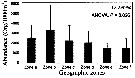
 Issued from : J.-S. Hwang, R. Kumar, H.-U. Dahms, L.-C. Tseng & Q.-C. Chen in Zool. Studies, 49 (2). [p.224, Fig.3). Issued from : J.-S. Hwang, R. Kumar, H.-U. Dahms, L.-C. Tseng & Q.-C. Chen in Zool. Studies, 49 (2). [p.224, Fig.3).
Average abundances of six Oithona species recorded in the South China Sea from Mar. 2000 to Oct. 2002.
Sampling stations between 16-24° N, 114-120° E.
These forms need confirmation. |
 Issued from : C. Castellani, P. Licandro, E. Fileman, I. Di Capua & M.G. Mazzocchi in J. Plankton Res., 2016, 38 (3). [p.706, Fig. 1]. Issued from : C. Castellani, P. Licandro, E. Fileman, I. Di Capua & M.G. Mazzocchi in J. Plankton Res., 2016, 38 (3). [p.706, Fig. 1].
Oithona similis monthly mean abundance (Ind./m3) at (a) English Channel: L4 (50°15' N, 4°13' W) between 1988 and 2013 and at (b) Gulf of Naples: LTER-MC (40°48.5' N, 14°15' E) between 1984 and 2013.
Sampled with WP2, by vertical net hauls from the sea floor (±55 m) to surface near Plymouth and zooplankton samples collected by vertical tows in the upper 50 m with a Nansen net; mesh apertures of the two nets: 200 µm. |
 Issued from : C. Castellani, P. Licandro, E. Fileman, I. Di Capua & M.G. Mazzocchi in J. Plankton Res., 2016, 38 (3). [p.707, Table 1]. Issued from : C. Castellani, P. Licandro, E. Fileman, I. Di Capua & M.G. Mazzocchi in J. Plankton Res., 2016, 38 (3). [p.707, Table 1].
Summary of Oithona similis annual mean and absolute range (min-max) of abundance (Ind./m3) and relative contribution (%) to total copepods at Plymouth (L4) and Gulf of Naples (LTER-MC) between 1988 and 2013. |
 Issued from : C. Castellani, P. Licandro, E. Fileman, I. Di Capua & M.G. Mazzocchi in J. Plankton Res., 2016, 38 (3). [p.708, Fig. 2]. Issued from : C. Castellani, P. Licandro, E. Fileman, I. Di Capua & M.G. Mazzocchi in J. Plankton Res., 2016, 38 (3). [p.708, Fig. 2].
Monthly mean (±SE) temperature (SST, °C), chlorophyll a concentration (Chl a, µg/l) and Oithona similis abundance (Ind./m3) measured at Plymouth (L4) and Gulf of Naples (LTER-MC) between 1988 and 2013.
Nota: For the authors, the abundance of O. similis at Plymouth was ± 10 times higher than in the Gulf of Naples, moreover this species had several peaks of abundance during the year at Plymouth but a single peak in spring in the Gulf of Naples. The two sites are characterized by similar chlorophyll a concentration, but different temperature.
The main mode of temporal variability in abundance was seasonal at both sites. The abundance was negatively correlated with sea temperature only in the Gulf of Naples, whereas it was positively correlated with Chl a at both sites. The authors conclude that the abundance of the species increases with prey availability up to 16°5 and that temperature > 20°C represents the main limiting factor for population persistence. |
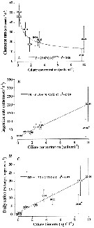
 Issued from : S. Zamora Terol in Tesis Doc. Univ. Politèc. Catalunya, 2013 [p.82-83, Table 3]. Issued from : S. Zamora Terol in Tesis Doc. Univ. Politèc. Catalunya, 2013 [p.82-83, Table 3].
Comparison of egg production and clutch sizes among different species of Oithona from field and lab studies.
b: egg per sac; d: maximum specific-egg production rate.
Also, see: Oithona attenuata, O. colcarva, O. davisae, O. nana, O. plumifera, O. setigera, O. aruensis, O. simplex. |
 Issued from : S. Zamora Terol in Tesis Doc. Univ. Politèc. Catalunya, 2013 [p.135, Fig. 7]. Issued from : S. Zamora Terol in Tesis Doc. Univ. Politèc. Catalunya, 2013 [p.135, Fig. 7].
Feeding rates of Oithona similis adult females on ciliates.
(A) Clearance rate (F, ml female-1 d-1.
(B) Ingestion rate (IR, cells female-1 d-1.
(C) daily ration (DR, % body carbon ingested female-1 d-1.
Each point represents the mean value (± SE) of 3-4 replicates
Cil-C: ciliate concentration, either cells or carbon.
Asterisk (*) indicates a date not included in the fitted equations, because the presence of negative values;
Equations used see Oithona davisae.
Sampling in Nuuk, Godthabsfjord (64°07' N, 51°53' W) in February-March, and Disko Bay (69°15'N, 53°33' W). Zooplankton samples collected by vertical hauls using WP2 (4-5 µm mesh aperture). |
 Issued from : G.A. Lopez-Ibarra, S. Hernandez-Trijillo, A. Bode & M.J. Zetina-Rejon in Cah. Biol. Mar., 2014, 55. [p.459, Fig.8]. Issued from : G.A. Lopez-Ibarra, S. Hernandez-Trijillo, A. Bode & M.J. Zetina-Rejon in Cah. Biol. Mar., 2014, 55. [p.459, Fig.8].
Abundance recorded in the geographic zones with the highest canonical coefficient on the first two axes of the discriminant analysis.
See informations and figures in Pleuromamma robusta from the same authors. |
 Issued from : T. Zuo, R. Wang, Ya-qu. Chen, Sh-wu Gao & Ke. Wang in J. Mar. Syst., 2006, 59. [p.169, Fig.9B]. Oithona similis Issued from : T. Zuo, R. Wang, Ya-qu. Chen, Sh-wu Gao & Ke. Wang in J. Mar. Syst., 2006, 59. [p.169, Fig.9B]. Oithona similis
Spatial of representative species abundance with isobaths shown in gray.
The circles are proportional in diameter to square root value of abundance.
Copepods collected vertically with plankton net (200 µm mesh aperture) from a depth near the bottom to the surface in autumn 2000 (18 October to 21 November).
Body length (mm): 0.75. |
 Issued from : C. Castellani, C. Robinson, T. Smith & R.S. Lanpitt in mar. Ecol/ Progr. Ser., 2005, 285. [p.131, Fig.2]. Issued from : C. Castellani, C. Robinson, T. Smith & R.S. Lanpitt in mar. Ecol/ Progr. Ser., 2005, 285. [p.131, Fig.2].
Oithona similis females from the English Channel (50°15'N, 04°13'W), between July and December 2003.
Weight-specific respiration rate (µl O2 mg C-1 d-1) versus temperature (T, °C) measured at in situ temperature (black circle) or after pre-conditioning at experimental temperature (empty circle).
Note logarithmic scaling.
The respiration rate of adult female was measured over the temperature range 4 to 25°C. The respiration rate changed exponentially with the temperature (ln O2-rate = - 3.59 + 0.114 T, r2 = 0.85, p < 0.001).
Over the temperature range examined, O. similis basic metabolic cost varied from a minimum of about 1.4 % body-C/day at 4°C to a maximum of 23 % body-C/day at 25°C, corresponding to an energy demand of about 3 % and 232 £% body-C/day respectively.
The Q10 = 3.1.
The respiration rate of O. similis from the study, is about 8 times lower than that of a calanoid of equivalent body weight estimated from published empirical metabolism-temperature data. For the authors, these differences in metabolic rates may account for the year-round persistence and higher abundances of Oithona spp. over calanoid, particularly in oceanic and oligotrophic environments where food resources may be limiting for calanoid copepods. |
 Issued from : C. Castellani, C. Robinson, T. Smith & R.S. Lanpitt in mar. Ecol/ Progr. Ser., 2005, 285. [p.132, Table 1]. Issued from : C. Castellani, C. Robinson, T. Smith & R.S. Lanpitt in mar. Ecol/ Progr. Ser., 2005, 285. [p.132, Table 1].
Oithona spp. Summary of respiration rates (range) reported in the litterature in different regions.
Nota: << The respiration rate of O. similis changed exponentially with temperature (ln O2-rate = - 3.59 + 0.114 T. Q10 = 3.1. Over the temperature range examined, O. similis basic metabolic cost varied from a minimum of about 1.4% body-C/day at 4°C to a maximum of 23% body-C/day at 25°C, corresponding to an energy demand of about 3% and 32% body-C/day respectively (i.e. assuming a respiratory quotient of 0.8 [for protein metabolism] and assimilation efficiency of 0.7 respectively (Ikeda & Motoda, 1978).
The respiration rate of O. similis in the English Channel, Station L4 (50°15'N, 04°13'W) is about 8 times lower than that of a calanoid copepod equivalent body weight estimated from publisher empirical metabolism-temperature data.
For the authors, these differences in lmetabolic rates may account for the year-round persistence and higher abundances of Oithona spp. over calanoids, particularly in oceanic and oligotrophic regions where food ressources may be limiting.
Success of Oithona spp. is its ability to feed on a wider size range and diversity of prey (see in Lampitt, 1978; Uchima, 1988; Gonzalez & Smetacek, 1994; Roff & al., 1995; Lonsdale & al., 2000) rather than to real differences in the metabolic rates between Oithona spp. and calanoids (Sabatini & Kiørboe, 1994; Nielsen & Sabatini, 1996).
The lower respiration rate may reflect different physiological, behaviourial and ecological adaptations from those of calanoids to live in the pelagial. Oithona spp. are ambush and coprophagus feeders, mostly drifting passively without generating a feeding current (Svensen & Kiørboe, 2000; Paffdenhöfer & Mazzocchi, 2002). Thus, whereas calanoids spend on average 80% of their time swimming, Oithobna spp. copepodites only move 0.9% or less of the time (Paffenhöfer, 1993; Hwang & Turner, 1995; Paffenhöfer & Mazzocchi, 2002). However, energy is expended not only in swimming speed, but also in the movement of mouth-parts. Thus, the lower metabolic rates of Oithona spp. could also be attributable to the absence of a feeding current.
Also, their smaller size, transparency and reduced motion probably make Oithona spp. less conspicuous than calanoids to both tactile and visual predators (Paffenhöfer, 1993; Atkinson & Snyder, 1997). Eiane & Ohman (2004) have shown that Oithona similis suffers lower mortality rates than Calanus finmarchicus and Pseudocalanus elongatus. >> |
 Issued from : J.-S. Hwang & J.T. Turner in P.S.Z.N. 1: Mar. Ecol., 1995, 16 (3). [p.209: Table 1, p.210: Table 2]. Issued from : J.-S. Hwang & J.T. Turner in P.S.Z.N. 1: Mar. Ecol., 1995, 16 (3). [p.209: Table 1, p.210: Table 2].
Table 1: Experimental protocol.
Table 2:Swimming versus non-swimming behaviour, and behavioural transitions per minute. Means (bold type), ranges, and standard deviations (SD). Number of repeated observations = 500.
Copepods collected in surface net from waters near Pitou (NE coast Taiwan: 25°N, 122°E) in daylight in July 1993.
Compare with Oithona nana, Temora turbinata, Oncaea venusta, Macrosetella gracilis and Undinula var. taiwanicus by the same authors. |
 Issued from : J.-S. Hwang & J.T. Turner in P.S.Z.N. 1: Mar. Ecol., 1995, 16 (3). [p.211: Figs.1, 2]. Issued from : J.-S. Hwang & J.T. Turner in P.S.Z.N. 1: Mar. Ecol., 1995, 16 (3). [p.211: Figs.1, 2].
Fig.1: A, Mean durations periods (seconds) of swimming versus non swimming behaviour by Oithona similis from north-east coast of Taiwan (near Pitou) in daylight in July 1993.
Fig.2: B, mean percentages of time allocated to swimming versus non-swimming behaviour by Oithona similis. |
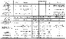
| | | | Loc: | | | Antarct. (Amundsen Sea, King George Is., Potter Cove, Peninsula, Croker Passage, Drake Passage, Scotia Sea, Weddell Sea, Patagonian Shelf, SW Atlant., Syowa station, Indian, Lützow-Holm Bay, Davis station-Gardner Is., Fletcher Lake, Ellis fjord, Pacif. (SW, S, SE), Ross Sea, Prydz Bay, McMurdo Sound, Bellingshausen Sea), sub-Antarct. Beagle Channel, (N South Georgia, Atlant. (SW, SE), off W Prince Edward, Crozet Is., Indian, Kerguelen Is. Pacif. (SW, S, SE), South Africa (E), Saldanha Bay, S Benguela Current, off E Tristan da Cunha, Namibia, Angola (Baia Farta), Congo, off S St. Helena Is., off Trinidade Is., off Ascension Is., Cape Verde Is., off Morocco-Mauritania, Cap Ghir, Canary Is., off Madeira, Patagonia, Peninsula Valdés, off Rio de la Plata, Brazil (off Macaé, Sao Joao, Rio de Janeiro, Campos Basin, Vitoria Bay, Vitoria-Cabo de Sao Tomé, Mucuri estuary, Camamu), Barbados Is., G. of Mexico, Cuba, Bermuda, New York Bight, Delaware Bay, Buzzards Bay, Long Island, Chesapeake Bay, Buzzards Bay, Woods Hole, Gulf of Maine, Massachusetts Bay, Georges Bank, Bay of Fundy, Browns Bank, Emerald Bank, Halifax, off SE & SW Nova Scotia, Bras d'Or Lake, Morrison's Pond, Shédiac Bay, Northumberland Strait, Bedford Basin, Saguenay fjord, upper St. Lawrence estuary, G. of St. Lawrence, Bradelle Bank, off E Newfoundland (Flemish Cap), Labrador, Tassiarsuk fjord, Godthaab Fjord, W Greenland, Godthabsfjord, N Baffin Sea, Baffin Sea (Lancaster Sound, W Baffin Bay), Smith Sound, Greenland Sea, Fram Strait, Kongsfjorden, Spitsbergen, Iceland, Faroe, Ireland, Lough Hyne, Norway Sea, Malangen fjord, Hardangerfjord, Akrefjord, Tromsø fjords, Nordvestbanken, White Sea, Barents Sea, Kola Bay, Franz Josef Land, Pechora Sea, Arct. (Ellesmere Is., Canadian abyssal plain, Nansen Basin, Amundsen Basin, Makarov Basin, off Alaska N, Barrow Srrait, Chukchi Sea, Beaufort Sea, off NW Alaska, Canada Basin, Kara Sea, Barents Sea, Lomonosov Ridge, Chupa Inlet, Laptev Sea), Bering Sea (slope and shelf), Karagin Bay, St. Lawrence Island, Anadyr Strait, Shpanberg Strait, North Sea, Gullmar Fjord, Elbe (estuaire), Bay of Kiel, Lübeck Bay, Gulf of Mecklenburger, Baltic Sea, Bornholm Basin, English Channel, Belon estuary, Arcachon Bay, off Bay of Biscay, S Bay of Biscay, Portugal, NW Spain, Mondego estuary, Galicia (coast), Ibero-moroccan Bay, off W Tangier, Medit. (M'Diq, Alboran Sea, Algiers, Gulf of Annaba, El Kala shelf, Castellon, Baleares, Banyuls, Thau Lagoon, Marseille, Toulon Harbour, Villefranche-s-Mer, Genoa, Ligurian Sea, Tyrrhenian Sea, G. of Naples, Strait of Messina, Gulf of Taranto, Taranto Harbour, NW Tunisia, G. of Gabès, Sfax, Adriatic Sea, mouth of Po, Ionian Sea, Aegean Sea, Thracian Sea, Marmara Sea, Black Sea, Sebastopol, Iskenderun Bay, Lebanon Basin, W Egyptian coast, Alexandria), Suez Canal, G. of Suez, Red Sea, Madagascar, Indian, India (Saurashtra coast, Mangalore coast, Pointcalimere-Manamelkudi, Gulf of Mannar, Palk Bay, Parangipettai coast), Bay of Bengal, Straits of Malacca, Indonesia-Malaysia, Sarawak: Bintulu coast, Philippines, China Seas (Bohai Sea, Yellow Sea, East China Sea, South China Sea), Xiamen Harbour), Taiwan Strait, off SW Taiwan,Taiwan (S, E, W, Kaohsiung Harbor, N: Mienhua Canyon, Pitou), Korea (E, S & W, Chunsu Bay), Korea Strait, Japan Sea, Japan (Honshu: Maizuru Bay, Tokyo Bay, Tanabe Bay, Yatsushiro-kai, Ariake Bay, Seto Inland Sea, Kyushu: Shijiki Bat, W Hokkaido), Pacif. NW & NE, Chukchi Sea, White Sea, Bering Sea, Aleutian Is., Beaufort Sea, Arch. New-Siberia, Alaska (Auke Bay), Station "P", British Columbia, Hecate Strait, Fjord system (Alice Arm & Hastings Arm), Portland Inlet, Vancouver Is., Dabob Bay, Friday Harbor, Oregon (coast, Yaquina Bay, off Newport), California, Mission Bay (San Francisco), Santa Monica Basin, Baja California (Bahia Magdalena, La Paz), Acapulco Bay, Tomales Bay, W Costa Rica, Clipperton Is., W & E Australia (North West Cape, Great Barrier, Brisbane River estuary, New South Wales, Melbourne), New Zealand (Kaikoura, Cape Farewell-Taranaki Bight, off Farewell Spit plume), Fidji Is., Ecuador, Peru, Chile (N-S, off Santiago, Concepcion), Strait of Magellan, Ushuaia.
The genetic and morphological differences show clearly that Oithona similis is not a truly cosmopolitan species, but a conglomerate of several cryptic species (see Wend-Heckmann, 2013). | | | | N: | 695 (??: see in remarks). | | | | Lg.: | | | (25) F: 0,95-0,75; (31) F: 1,2-1,15; (34) F: 0,93-0,9; (35) F: 1,08-0,76; (36) F: 0,92-0,8; (45) F: 0,95-0,7; M: 0,7-0,6; (59) F: 0,96-0,69; M: 0,7-0,5; (66) F: 1,05-0,71; M: 0,82-0,75; (46) F: 0,8-0,73; M: 0,61-0,59; (104) F: 0,82; (109) F: 0,8-0,72; M: 0,63-0,5; (114) F: 1,02-0,8; M: 0,7; (116) F: 0,84; M: 0,65; (133) F: 0,9-0,7; M: 0,6-0,5; (141) F: 0,9-0,7; M: 0,6-0,5; (155) F: 0,84-0,69; M: 0,65-0,6; (190) F: 0,86; M: 0,78; (208) F: 0,8-0,7; M: 0,75-0,73; (246) F: 0,81-0,76; (254) F,M: 1; (334) F: 0,95-0,7; M: 0,7-0,5; (354) F: 0,75-0,68; (373) F: 0,99-0,68; M: 0,75-0,58; (432) F: 1-0,75; (449) F: 0,96-0,73; M: 0,7-0,59; (627) F: 0,96-0,68; (649) F: 0,78; M: 0,67; (796) F: 0,86-0,69; (880) F: 0,78; M: 0,6-0,7; (991) F: 0,68-0,96; M: 0,6-0,7; (1239) F: 0,65-0,86; (1302) F: 0,430-0,533; M: 0,428-0,493; (1232) F: 0,64-1; M: 0,6-0,7; {F: 0,44-1,20; M: 0,43-0,82}
Probably F = 0,44, and male = 0,43 belonging to another species that O. similis s.s. | | | | Rem.: | epi- to bathypelagic.
Sampling depth (Antarct., sub-Antarct.) : 0-1000 m.
For jespersen (1939, p.79) this species is one of the most frequently occurring copepods in the East Greenland fjords.
Although the geographical distribution of this species seems cosmopolite, the list of studied authors shows that cold septentrional (northern) waters and Antarctic waters are preferable localities, even at a latitude of Taiwan (cf. Hsieh & al., 2004 (p.398, tab.1 & fig.2).
Observed in ballast waters of ships at San Francisco.
Remark concerning Oithona helgolandica: The rough description of Oithona helgolandica was done from a male found near Helgoland, the female was never described other than by synonymy with O. similis Claus, 1866. The opinion put forward by Sars (1918, p.207) seems well founded. Under these conditions, the arguments developed by Crisafi (1959) are not retained, and this species is considered as doubtful or a synonym of O. nana as formulated by Rosendorn (1917) and Sars (1918). Nishida & al., 1977 (p.151) consider this form as doubtful. Also the authors after Claus (1863) who cite this form refer most often to Oithona similis.
For Dvoretsky & Dvoretsky (2011, p.129) the mortality rate was significantly higher in the White Sea than in the Barents Sea. The salinity in the White Sea is lower than in the Barents Sea. Five hydrological areas were revealed in the Barents Sea and four hydrological areas in the White Sea.
After Dvoretsky & Dvoretsky (2009 c, p.165) the average body size is correlated negatively with temperature and positively with salinity, while total A1 length , total number of setae, total setae length and relative A1 length correlated negatively with salinity and positively with temperature. These data have an adaptative significance. Gaudy (1971 a) shows a relation between the size and the length of the antennula, linked with the water density in the Gulf of Marseille for Centropages typicus.
For Wend-Heckmann (2013) the genetic and morphological differences show clearly that Oithona similis is not a truly cosmopolitan species, but a conglomerate of several cryptic species. This opinion is agreed by Cepeda & al. (2016, p.1); the authors strongly recommend specifically reporting the authority upon wgich the identification of either O. similis s.l. or O. helgolandica s.l. has been undertaken. In this process, particular reference should be made for female specimens in respect to: (1) relative antennule length, (2) presence/absence of the small distal outer spine on exopod segment 3 of leg 4, (3) endopod segmentation of leg 1. There are not conclusive fundamentals at present in support of an objective synonymy between O. similis and O. helgolandica. Species should not be renamed or newly assigned based on morphology alone without the support of molecular genetic sequence information.
Zaika (1968), nearshore in Black Sea, finds a daily ratio P/B = .04 d-1 and an annual P/B yr-1 = 16.
After Benedetti & al. (2018, p.1, Fig.2) this species belonging to the functional group 6 corresponding to small ambush feeding omnivorous.
Ohtsuka & Nishida (2017, p.578) consider this species as a cold-water species on the japanese coasts infuenced by Oyashio waters.
Madoui & al. (2017) consider O. similis s.s. as amphitropical;
After Karnovsky & al., 2003 (p.289, Appendix 2) the mean dry mass (mg) female is 0.003.
See in DVP Conway & al., 2003 (version 1) | | | Last update : 28/10/2022 | |
|
|
 Any use of this site for a publication will be mentioned with the following reference : Any use of this site for a publication will be mentioned with the following reference :
Razouls C., Desreumaux N., Kouwenberg J. and de Bovée F., 2005-2024. - Biodiversity of Marine Planktonic Copepods (morphology, geographical distribution and biological data). Sorbonne University, CNRS. Available at http://copepodes.obs-banyuls.fr/en [Accessed April 26, 2024] © copyright 2005-2024 Sorbonne University, CNRS
|
|
|
|

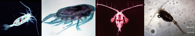


;)
;)
;)
;)
;)
;)
;)
;)
;)
;)
;)
;)
;)
;)
;)
;)
;)
;)
;)
;)
;)
;)
;)
;)
;)
;)
;)
;)
;)
;)
;)
;)
;)

;)
;)
;)
;)
;)
;)
;)
;)
;)
;)
;)
;)
;)
;)
;)
;)
;)
;)
;)
;)
;)
;)
;)
;)
;)
;)
;)
;)
;)
;)
;)
;)