|
|
 |
|
Calanoida ( Order ) |
|
|
|
Diaptomoidea ( Superfamily ) |
|
|
|
Temoridae ( Family ) |
|
|
|
Eurytemora ( Genus ) |
|
|
| |
Eurytemora affinis Poppe, 1880 (F,M) | |
| | | | | | | Syn.: | Temora inermis Boeck,1864;
Eurytemora hirundindo Giesbrecht, 1881 (p.257); 1882 (p.152); Harder, 1968 (p156, Table 1, 6, behaviour vs. density discontinuity);
Eurytemora hirundoides : Sars, 1902 (1903) (p.102, Figs. F, M,); Breemen, 1908 (p.101, fig.); Sharpe, 1910 (p.410, fig. 3); Esterly, 1924 (p.93, figs.F,M); Grice, 1960 (p.220); Raymont Carrie, 1964 (p.195); Carter, 1965 (Rem.: p.351); Faber, 1966 (p.191, 193, Rem.); Maclellan D.C., 1967 (p.101, 102: occurrence); Corkett & McLaren, 1970 (p.161, development rate egg-CI); Lefèvre-Lehoërff, 1972 (p.1681); Yassen, 1973 (p.1, rearing, biology); Landry, 1975 a (p.434, Rem.: p.437, fig.3); Kos, 1976 (Vol. II, figs.F,M); Gyllenberg, 1980 (p.181, feeding); 1984 (p.229, feeding-bacteria); Vuorinen & al., 1983 (p.62, fig.1, Table 1: predation & vertical migration); Poli & Castel, 1983 (p.79, biological cycle); De Ladurantaye & al., 1984 (p.21, fig.5, advective processes in fjord); Citarella, 1989 (p.123, abundance); Shih & Marhue, 1991 (tab.3); Boxshall & Halsey, 2004 (p.208: figs.F,M); Dvoretsky & Dvoretsky, 2011 b (p.469, Table A, abundance, biomass); Barton & al., 2013 (p.522, table 1: metabolism, feeding mode, biogeo);
Eurytemora affinis hirundoides : Castel & Veiga, 1990 (p.119);
Temorella affinis : Canu, 1892 (p.173);
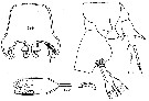
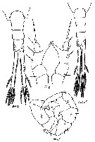
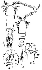
Temorella affinis hispida Nordquist, 1888 | | | | Ref.: | | | De Guerne & Richard, 1889 (p.562: tableau); van Breemen, 1908 a (p.101, Rem.); Labbé, 1927 (p.204, figs.M, F); Gurney, 1931 a (p.202, figs.F,M); Wilson, 1932 a (p.111, figs.F,M); Rose, 1933 a (p.173, figs.F,M); Dussart, 1967 (p.73, figs.F,M); Shih & al., 1971 (p.46); Katona, 1971 (p.5, Descr.N, juv., figs.N, juv., F,M); Kos, 12976 (Vol. II, figs.F,M); Heron & Damkaer, 1976 (p.128, 129, Table 1: synonymy, 2: ratio anal segment/uropods); Gardner & Szabo, 1982 (p.314, figs.F,M); Schnack, 1982 (p.89, figs.Mx2, Md, Mxp); Dussart & Defaye, 1983 (p.47); Chihara & Murano, 1997 (p.917, Pl.181: F,M); Hoffmeyer & al., 2000 (p.111, Rem.); Lee, 2000 (p.2014, reproductive isolation); Lee & Frost, 2002 (p.111, species complex, phylogeny); G. Harding, 2004 (p.19, figs.F,M); Rasch & al., 2004 (p.559, genome size); Ferrari & Dahms, 2007 (p.63, 83, Rem., Table XVII, XVIII); Winkler & al., 2008 (p.415, genetic analyses); Dodson & al., 2010 (p.653, table 1, 2, fig.4, 5, 6, key Female: p.146, Rem.); Soussi & al., 2010 (p.851, figs.1, 2, 3, 4, 5, 6, 7: intersexuality); Winkler & al., 2011 (p.1841, figs. 2, 3, 5, mtDNA haplotype frequencies vs geographic regions); Xuereb & al., 2012 (p.457, Mol. Biol.); Alekseev & Souissi, 2011 (p.41, fig.9: F, M, Rable 2, 3, 4, Rem.); Sukhikh & Alekseev, 2013 (p.85, Rem: Complex of cryptic species, Table 1, 2, Fig.11, 12, Key of species); Laakmann & al., 2013 (p.862, figs.1, 2, 3, 4, 5, Table 1, 2, 3, mol. Biol.); Kos, 2016 (p.55, figs.F, M, Rem.); Sukhikh & Akekseev, 2013 (p.85, Rem.: complex-species, Table 1, 2, fig.2, 11, 12,key F, M); Ohtsuka & Nishida, 2017 (p/576, Rem.) | 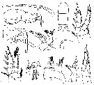 issued from : C.O. Esterly in Univ. Calif. Publs Zool., 1924, 26 (5). [p.94, Fig.F). As Eurytemora hirundoides. Female (from San Francisco Bay): 1, A1; 2, habitus (lateral); 3, cephalothorax (dorsal); 4, P2; 5, last thoracic segment and urosome (lateral); 6, A2; 7, forehead (obliquely from ventral); 8, P3; 9, last thoracic segment and urosome (dorsal), with spermatophores; 10, Md; 11, P5; 12, P1.
|
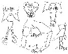
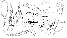 issued from : C.O. Esterly in Univ. Calif. Publs Zool., 1924, 26 (5). [p.95, Fig. G). As Eurytemora hirundoides. Male:1, habitus (dorsal); 2, P4; 3, P3; 4, two segments of A1 proximal to geniculation, and the one distal to it; 5, Mx2; 6, Mxp; 7, A2; 8, right A1; 9, P5 (left foot at left of drawing).
|
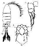
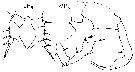 issued from : G. Harding in Key to the adullt pelagic calanoid copepods found over the continental shelf of the Canadian Atlantic coast. Bedford Inst. Oceanogr., Dartmouth, Nova Scotia, 2004. [p.19]. Female & Male.
|
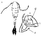
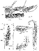 issued from : A. Labbé in Archiv. Zool. Exp. Génér., 1927, 66 (4). [p.204, Figs.194-198]. Male (from Le Croisic): 194, right A1; 195, same (sense organs in lateral view); 196, same (face view); 197, optical cross-section of sense organs; 198, nerves showed after preparation with nethylen blue coloration (below and inside the sense organ).
|
 issued from : A. Labbé in Archiv. Zool. Exp. Génér., 1927, 66 (4). [p.205, Figs.199-201]. Female (from Le Croisic): 199, genital apertures; 201, last thoracic segment with P5 and genital segment with 2 spermatophores. Male: anterior part of spermatophore with spoon-like end.
|
 Issued from : B. Dussart les Copépodes des eaux continentales d'Europe occidentale, Rdit. B. Boubée & Cie, Paris., 1967, I. [p.73, Fig.16].
Female & Male: a, after Gurney (1931).
Female: b, after Poppe (1880).
|
 Issued from : M. Chihara & M. Murano in An Illustrated Guide to Marine Plankton in Japan, 1997. [p.919, Pl. 181, fig.283 a-c]. Female : a, habitus (dorsal); b, P5; c, P1. Note characteristics numbered 1, 2, 3 into circles.
|
 Issued from : M. Chihara & M. Murano in An Illustrated Guide to Marine Plankton in Japan, 1997. [p.919, Pl. 181, fig.283 a-b]. Male: a, habitus (dorsal); b, P5. Note characteristics numbered 1, 2, 3 into circles.
|
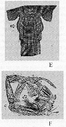 Issued from : V.R. Alekseev & A. Souissi in Zootaxa, 2011, 2767. [p.53, Fig.9, E, F]. Eurytemora affinis (Poppe, 1880) (Photo: Mrs N. Sukhikh): E, female genital somite with out wing-like outgrowth; F, male P5 with arrow indicating left basipod. Nota: Compare with Eurytemora carolleeae Alekseev & Souissi, 2011, cryptic species from NE USA estuaries.
|
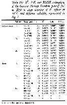
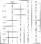
 Issued from : V.R. Alekseev & A. Souissi in Zootaxa, 2011, 2767. [p.51, Table 2]. Selected morphometric indexes in females of E. carolleeae Alekseev & Souissi, 2011 (cryptic species from NE USA coast) and E. affinis (Poppe, 1880) from their type localities. Mean + standard deviation (Min-Max). In bold- significant difference with p<0.05. * Only in one female among 56 examined, possibly an aberrant specimen.
|
 Issued from : V.R. Alekseev & A. Souissi in Zootaxa, 2011, 2767. [p.51, Table 3]. Selected morphometric indexes for E. carolleeae Alekseev & Souissi, 2011 (cryptic species from NE USA coast) and E. affinis (Poppe, 1880) in males from their type localities. Mean + standard deviation (Min-Max).
|
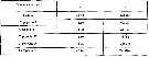
 Issued from : V.R. Alekseev & A. Souissi in Zootaxa, 2011, 2767. [p.51, Table 4]. Selected morphometric indexes in female and male of E. carolleeae Alekseev & Souissi, 2011 (cryptic species from NE USA coast) and E. affinis (Poppe, 1880) from several European localities).
|
 Issued from : V.R. Alekseev & A. Souissi in Zootaxa, 2011, 2767. [p.55, Table Fig. 10]. Morphological indexes in E. carolleeae Alekseev & Souissi, 2011 (cryptic species from the Chesapeake Bay, USA and St. Lawrence Bay, Canada) and E. affinis (Poppe, 1880) from their type locality. Males: Index P4, distal spine/segment length ratio in Exp P4; Index P5, L/W ratio in Bas P5 left.
|
 Issued from : M.S. Kos in Zoological Institut RAS, St. Petersburg, 2016, 179, [p.56, Fig.24]. Eurytemora affinis female and male from the Baltic Sea.
|
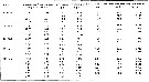
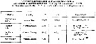
 Issued from : N.M. Sukhikh & V.R. Alekseev in Proc. Zool. Inst. RAS, 2013, 317 (1). [p.87, Table 1]. Morphometric indexes in females Eurytemora affinis; E. caspica, E. carolleeae from the type localities: Elbe River, North Caspian Sea and Chesapeake bay and . Mean ± error of the mean (Min-Max).
|
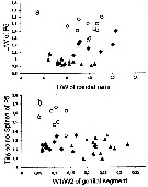
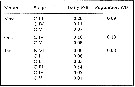
 Issued from : N.M. Sukhikh & V.R. Alekseev in Proc. Zool. Inst. RAS, 2013, 317 (1). [p.88, Table 2]. Morphometric indexes in males Eurytemora affinis from the Elbe Estuary (triangles); E. caspica from the Caspian Sea (squares), E. carolleeae from the Chesapeake Bay (rings). a : males, b: females.
See Tables 1 and 2.
|
 Issued from : N.M. Sukhikh & V.R. Alekseev in Proc. Zool. Inst. RAS, 2013, 317 (1). [p.97, Fig. 11]. Morphological indexes in Eurytemora affinis; E. caspica, E. carolleeae from the type localities: Elbe Estuary, North Caspian Sea and Chesapeake bay and . Mean ± error of the mean (Min-Max).
|
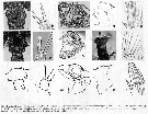 Issued from : N.M. Sukhikh & V.R. Alekseev in Proc. Zool. Inst. RAS, 2013, 317 (1). [p.98, Fig. 12]. Main differences between Eurytemora affinis (Poppe, 1880): a-e; E. carolleeae: f-j and E. caspica : k-o.
a, f, k : female genital somite; b, g, l : distal segment of female P5 and tiny spine (arrow indicating); c, h, m : male P5 with ellips indicating left basipod; d, i, n : male Md (arrow indicating a gap); e, j, o : setae of swimming legs with arrow indicating segmentation.
|
 Issued from K.M. Sukhikh & V.R. Alekseev in Proc. Zool. Inst. RAS, 2013 (p.97, 99). Females :1 - In P5, tiny spine about 10% or less of length of nearest lateral spine, shorter than width of nearest distal spine in insertion place ............. 2
1 - In P5, tiny spine about 15-30% of length of nearest lateral spine, equal to width of nearest distal spine in insertion place ....... E. affinis.
2 - Mandible (Md) with more or less zqual teeth; outside tooth not separated from neighboring teeth by gap; caudal setae without clearly seen segment-like divisions ........ E. caspica.
2 - Mandible (Md) with outside tooth clearly separated from neighboring teeth by gap; caudal setae with clearly seen segment-like division ....... E. carolleeae. Males :1 - Caudal rami always with spines on dorsal surface (sometimes few). In left P5 basipodite with maximal width in anterior part of lateral outgrowth and with length/width ratio usually less thanj 1 ....... E. affinis. 1 - Caudal rami always naked on both dorsal and ventral sides. Left P5 basipodite with maximal width in the middle part, with length/width ratio usually more than 1 (see Table 2, Fig. 10) ....... 22 - Mandible (Md) wiyh more or less equal teeth; outside tooth not separated from neighboring teeth by gap; caudal setae without clear seen segment-like separation ....... E. caspica. 2- Mandible (Md) with outside tooth clear separated from neighboring teeth by gap; caudal setae with distinct segment-like separation ........ E. carolleeae.
|
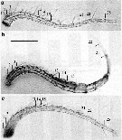 Issued from : A. Souissi, S. Souissi, D. Devreker & J.-S. Hwang in Ma. Biol., 2010, 157. [p.857, Fig. 4]. Different types observed of antennule: of normal female (a), of normal male (b), and feminized male (c). Numbers show the first three segments (1-3), segments 13-15, and segments 21-22. The last segment 25 in normal female (a) and feminized male (c) is also labeled. The measurements of the 15th segment in the geniculated antennules (b) are shown by arrows. Scale bar:= 200 µm. Nota: The prosome size and antennules of intersex individuals are similar to those of normal females, but all the other morphological details are more similar to normal males.
|
 Issued from : A. Souissi, S. Souissi, D. Devreker & J.-S. Hwang in Ma. Biol., 2010, 157. [p.858, Fig. 6]. Different types observed of P5 of normal female (a), of normal male (b) and of feminized male (c). The sizes of the basipodite of the left P5 were taken as shown with arrows (in b-c) Scale bar = 100 µm.
|
 Issued from : S.I. Dodson, D.A. Skelly & C.E. Lee in Hydrobiologia, 2010, 653. [p.141, Table 2]. Descriptions of North American species of Eurytemora from Alaska. PX1: indicates the first (basal ) exopodal segment of P5.
|
 Issued from : M.S. Kos in Field guide for plankton. Zool Institute USSR Acad., Vol. II, 1976. As Eurytemora hirundoides Sars, 1903. Female: 1, habitus (dorsal), with eggs; 2, P5. Male: 3, habitus (dorsal); 4, P5.
| | | | | Compl. Ref.: | | | Deevey, 1960 (p.5, Table II, fig.8: annual abundance); H. Schulz, 1961 (p.57); Engel, 1962 (p.252, american occurrences); Northcote & al., 1964 (p.1069, Table II); Dimov, 1964 a (p.31); Heinle, 1969 (p.186, temperature effect); 1969 a (p.150, Table 1, culture); Katona, 1970 (p.373, generation times, sex ratios, reproduction, survival vs. temperature); 1973 (p.574, Table 1, 2, fig.1, sex pheromones); Eriksson, 1973 a (p.95, fig.8, area abundance distibution); Katona, 1975 (p.89, Table 1I, II, figs., copulation, egg production); Bradley, 1975 (p.26, t° & Sal. effects); Heinle & Flemer, 1975 (p.235, carbon requirements); Richman & al., 1977, (p.69, grazing: particle selection); Allan & al., 1977 (p.317, grazing); Heinle & al., 1977 (p.341, feeding, egg production); Harris & al., 1977 (p.187, polluant effect); Berdugo & al., 1977 (p.138, reproduction vs pollution); Ott & al., 1978 (p.49, toxic effect); Bradley, 1978 (p.177, temperature acclimatation); Knatz, 1978 (p.68, Table 1, fig.3, abundance, %); Collins & Williams, 1981 (p.273, monthly distribution-salinity); Grice & Marcus, 1981 (p.125, Dormant eggs, Rem.: p.135); Burkill & Kendall, 1982 (p.21, production); Boak & Goulder, 1983 (p.139, Rem.: bacterioplankton); Jacoby & Youngbluth, 1983 (p.84, Table 4, Rem: mating); Barthel, 1983 (p.269, filtration, ingestion, respiratory rates); Tremblay & Anderson, 1984 (p.6, Rem.); Roddie & al., 1984 (p.191, S-T tolerance & osmoregulation); Tremblay & Anderson, 1984 (p.6), Rem.); Williams & Collins, 1985 (p.28); Bradley, 1986 (p.561, genetic/temperature/salinity); Kankaala & Johansson, 1986 (p.1027, length-biomass); Heckman, 1986 (p.176, anadromus migration); Vuorinen & Ranta, 1987 (tab.2, 4); Sellner & Bundy, 1987 (p.1435, turbidity effects); Giguère & al., 1989 (p.522, Table 1, formaldehyde preservation); Castel & Feurtet, 1989 (p.577, population dynamic); Stoecker & McDowell Capuzzo, 1990 (p.891, feeding); Jouffre & al., 1991 (p.489, lagoon); Naess, 1991 (p.261, fig.6, 7, resting egg); Bradley & Davis, 1991 (p.321, survival vs. temperature & genetic); Bradley & al., 1992 (p.3, molecular biology); Hough & Naylor, 1992 (p.27, endogenous rhythms); Viitasalo, 1992 (tab.2); Hirche, 1992 (p.395, Table 1, egg production, k-sreategy); Ban, 1992 (p.361, diapause, egg production vs environmental factors); Ban & Minoda, 1992 (p.51, hatching of diapause eggs); Pietsch, 1993 (p.215, mortality rates); Escaravage & Soetaert, 1993 (p.201, development vs. t°, secondary production); Castel, 1993 (p.145, long-term annual distribution); Ban, 1994 (p.721, temperature & food concentration effects); Ban & Minoda, 1994 (p.185, diapause egg production); Marcus & al., 1994 (p.154, Rem. p.157); Sellner & al., 1994 (p.249); Hoffmeyer, 1994 (p.303); Pietsch, 1995 (p.127, production); Irigoien & al., 1996 (p.163, gut clearance rate); Madhupratap & al., 1996 (p.77, Table 2: resting eggs); Ban S, Burns C. & al., 1997 (p.287, fig.1, Table 1, 2, feeding, reproduction); Cordell & al., 1997 (p.7, % change vs. 1980-1997); Suarez-Morales & Gasca, 1998 a (p.111); Mauchline, 1998 (tab.8, 18, 21, 26, 33, 35, 40, 45, 46, 47, 48, 51, 56, 58, 61, 62, 63, 65); Hairston & Bohonak, 1998 (p.23, Table 3); Viitasalo & al., 1998 (p.129, behaviour vs. predator): Gasparini & Castel, 1999 (p.877, diet); Gasparini & al., 1999 (p.195, egg production); Harvey & al., 1999 (p.1, 49: Appendix 5, in ballast water vessel); Lee, 1999 (p.1423, invasive); Ueda & al., 2000 (tab.1); Peitsch & al., 2000 (p.175, seasonal-long term abundances vs. transect); Burdloff & al., 2000 (p.165, egg production); Holmes, 2001 (p.27); Miramand & al., 2001 (p.1056, matals concentration); Kimmel & Bradley, 2001 (p.135, protein expression vs Salinity-temperature variation); Mouny & Dauvin, 2002 (p.13, fig.3, 5, 6, Table 4); Tackx & al., 2003 (p.305, feeding); Titelman & Kiørboe, 2003 a (p.137, nauplius behaviour); Lee & Petersen, 2003 (p.296, acclimatization); Forget-Leray & al., 2005 (p.268, toxicity vs development); Cordell & al., 2007 (p.218, fig.7); David & al., 2007 (p.377); 2007a (p.429, figs.2, 4, 5, Table 2, 3, 4, 5, 6); Cailleaud & al., 2007 (p.270, contamination); 2007 a (p.281); Devreker & al.,2007 (p.1117, post-embryonic development vs t°, Sal.); 2008 (p.1329), tidal effects); Höök & al., 2008 (p.29); Darnis & al., 2008 (p.994, Table 1); Suarez-Morales & al., 2008 (p.679, occurrence); Devreker & al., 2008 (p.1329, abundance vs tidal estuary); Devreker & al., 2009 (p.113, reproduction vs t° & Sal.); Beyrend-Dur & al., 2009 (p.713, table II, development time, reproduction, vs salinity); Devreker, 2009 (p.113, reproduction vs temperature & salinity); Brylinski, 2009 (p.253: Tab.1, p.255: Rem.); Cailleaud & al., 2009 (p.64, contaminant effects); Telesh & al., 2009 (p.16, fig.2.1, p.18: Table 2.1); Dur & al., 2009 (p.1073, reproduction); Seuront, 2010 (p.1223: salinity effect); Souissi & al., 2010 (p.1227: salinity effect); Michalec & al., 2010 (p.805); Mialet & al., 2010 (p.116); Devreker & al., 2010 (p.245); Modéran & al., 2010 (p.219, seasonal distribution); Dvoretsky & Dvoretsky, 2010 (p.991, Table 2); Bollens & al., 2011 (p.1358, Table III, fig.8); Strasser & al., 2011 (p.1210, fecundity model vs environment); Schmitt & al., 2011 (p.773, Rem.: behavior); Steele C.W. & Scarfe, 2011 (p.142, model courtship/copulation vs population density); Cailleaud & al., 2011 (p.228, behavior); Dur & al., 2011 (p.197, behavior); Elliot & Tang, 2011 (p.1039, spatial & temporal distribution); Mahjoub & al., 2011 (p.1095, vulnerability to predator); Sakaguchi & al., 2011 (p.18, Table 2, occurrences); Sopanen & al., 2011 (p.1564, mortality vs algal toxicity); Cailleaud & al., 2011 (p.226, contaminant bioconcentration); Glippa & al., 2011 (p.255, resting eggs); Postel, 2012 (p.327, Table 1); Delpy & al., 2012 (p.1921, Table 2); DiBacco & al., 2012 (p.483, Table S1, ballast water transport); Stefanova & al., 2012 (p.403, Table 2, interannual abundance); Drillet & al., 2012 (p.155, Table 1, culture); Bollens & al., 2012 (p.101, Table 1, species competition); Vehmaa & al., 2012 (p.351, reproduction vs algal composition); Madéran & al., 2012 (p.126, feeding adaptation vs turbidity); Devreker & al., 2012 (p.72, development, egg production); Holliland & al., 2012 (p.298, diel vertical migration); Arula & al., 2012 (p.33, Table 2: interannual abundance); Loick-Wilde & al., 2012 (p.199, feeding, N2 incorporation); Gusmao & al., 2013 (p.279, Table 3, 4, sex-specific predation by fish, fig.3: sex ratio vs temperature); Dur & al., 2013 (p.21, population dynamics model); Gissi & al., 2013 (p.86, Table 3, copper toxicity); Gorokhova & al., 2013 (p.1, pigmentation vs predation); Souissi & al., 2013 (p.38, behavior vs ciliate epibionts); Seuront, 2013 (p.724, mate-feeding behaviour); Michalec & al., 2013 (p.129, behavior vs aquatic toxics); Lesueur & al., 2013 (p.60, survival, growth vs toxicity); Lloyd & al., 2013 (p.299, egg production); Bradley C.J. & al., 2013 (p.49, swimming behavior); Setälä & al., 2014 (p.77, table 1, fig.1, microplastic ingestion); Kimmerer & al., 2014 (p.722, reproduction , growth vs food); Buskey & al., 2017 (p.754, amyelinate fiber vs escape response); Hansen B.W. & al., 2017 (p.984, pH effects); Baumgartner & Tarrant, 2017 (p.387, resting eggs, Rem.); Richirt & al., 2019 (p.3, Table 1, fig.2, 3, 4, 5, abundance changes vs years 1998-2014, table 2: diversity index) | | | 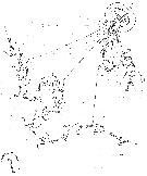 issued from : S.K. Katona in Limnol. Oceanogr., 1973, 18 (4). [p.578, Fig.1] issued from : S.K. Katona in Limnol. Oceanogr., 1973, 18 (4). [p.578, Fig.1]
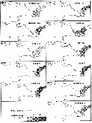
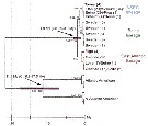
Diagram of mate-seeking in Eurytemora affinis (from Bar Harbor, Maine).
1: Short, successful search; 2: Male fails to locate distant female in long search; 3: Male is too far away from female to detect her.
Scattered dots represent the concentration gradient of hypothetical chemical attractant. |
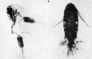 issued from : S.K. Katona in Crustaceana, 1975, 28 (1). [Pl. 1]. issued from : S.K. Katona in Crustaceana, 1975, 28 (1). [Pl. 1].
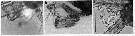
Eurytemora affinis. 1, two males have seized the same female (photograph by Ian Riddell); 2, female with about 2 spermatophores attached.Nota: A male first seizes a female by her posterior abdomen or caudal rami using his geniculate right antennule. Seizure of a female's antennule or swimming legs occasionally occurs. Several males sometimes seize a single female, but only one copulate with her at one time. Seizure can last for from 30 secondes to over an hour. Females commonly bear more than one spermatophore. Observations suggest that they resulult from a series of matings with males, rather than from a single prolonged mating. |
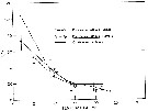 issued from : S.K. Katona in Helgol. Meersunt., 1970, 20. [p.376, Fig.1]. issued from : S.K. Katona in Helgol. Meersunt., 1970, 20. [p.376, Fig.1].
Generation times (± 2 SD) in 20 p.1000 salinity sea water at different temperatures.
W.H.O.I.: culture started with females taken from Oyster Pond, a fresh brackish pond near Woods Hole (Massachussets)
Hamble: Culture from the Hamble River at Southampton (England)
For E. herdmani from Nahant (Massachussets). |
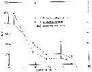 issued from : S.K. Katona in Helgol. Meersunt., 1970, 20. [p.379, Fig.3]. issued from : S.K. Katona in Helgol. Meersunt., 1970, 20. [p.379, Fig.3].
Average survival times and maximum observed survival times for females in 20 p.1000 salinity sea water at different temperatures and with an excess food.
After Katona, the survival times presented here probably underestimate the potential lifetimes in nature [but without predator. CR] |
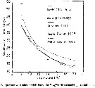
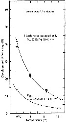 Issued from : C.J. Corkett & I.A. McLaren in J. mar. biol. Ass. U.K., 1970, 50. [p.164, Fig.I]; Issued from : C.J. Corkett & I.A. McLaren in J. mar. biol. Ass. U.K., 1970, 50. [p.164, Fig.I];
Development times of eggs to harching and between hatching and appearance of copepodite I in abundant food at the different temperatures. The points are means for eggs and individuals for older stages.
Individuals of Eurytemora hirundoides (= E. affinis) from waters near Halifax (Nova Scotia) raised in vials with an excess of food (Isochrysis galbana) at several controlled temperatures (See in Corkett, 1967). |
 issued from : N.R. Collins & R. Williams in Mar. Biol., 1981, 64. [p.276, Fig.5]; issued from : N.R. Collins & R. Williams in Mar. Biol., 1981, 64. [p.276, Fig.5];
Eurytemora affinis. Monthly distribution and abundance in Bristol Channel and Severn Estuary from November 1973 to February 1975, together with 30 p.1000 S isohaline. |
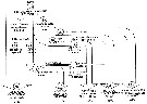 Issued from : M. Viitasalo, T. Kiørboe, J. Flinkman, L.W. Pedersen & A.W. Visser in Mar. Ecol. Prog. Ser., 1998, 175. [p.134, Fig.3]. Issued from : M. Viitasalo, T. Kiørboe, J. Flinkman, L.W. Pedersen & A.W. Visser in Mar. Ecol. Prog. Ser., 1998, 175. [p.134, Fig.3].
Gasterosteus aculeatus vs Eurytemora affinis. Flow chart of the 137 predatory interactions in Expts 2A and 2B. Encircled numbers refer to the absolute number of interactions of each type; percentages are given as percentages of the total number of interactions. |
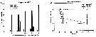 Issued from : S. Sopanen, O. Setala, J. Piiparinen, K. Erler & A. Krem in J. Plankton Res., 2011, 33 (10). [p.1568, Figs. 2, 3]. Issued from : S. Sopanen, O. Setala, J. Piiparinen, K. Erler & A. Krem in J. Plankton Res., 2011, 33 (10). [p.1568, Figs. 2, 3].
Fig.2 (left side): Condition of the copepods E. affinis (shown as percentage of all copepods in each experiment)after 24h exposure to dinoflagellate Alexandrium ostenfeldii cell suspensions at different cell concentrations (50-1200 cells mL). The copepod condition is ranked based on observations on their behavorial and movement.
Fig.3 (right side): Condition of the copepods A. affinis exposed to A. ostenfeldii cell suspensions at different concentrations through time. The copepod condition is ranked based on observations on their behavior and movement. The condition ranks (0-3) used are 0 = dead, 1 and 2 = impaired, 3 = normal. Dotted line: animals incubated in sea water controls. Error bars represent standard deviation. |
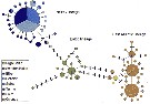 Issued from : G. Winkler, S. Souissi, C. Poux & V. Castric in Mar. Biol., 2011, 158. [p.1846, Fig.2]. Issued from : G. Winkler, S. Souissi, C. Poux & V. Castric in Mar. Biol., 2011, 158. [p.1846, Fig.2].
Parsimony mtDNA haplotype network for the European E. affinis populations.
Circle size is proportional to haplotype frequency. The smallest and the biggest circle represent one of 93 individuals. Black bars reptesent missing haplotypes. Colors indicate the geographic origin of haplotypes.
Nota: To gain information on genetic subdivision and to evaluate heterogeneity among European populations were analysed from 8 locations from 58° to 45°N and 0° to 23°E, using 549 base pairs of the mitochondrial cytochrome oxidase subunit I (COI) gene.
These geographically separated lineages showed sequences divergence of 1.7-2.1 % dating back 1.9 million years (CI: 0.9-3.0 My) with no indication of isolation by distance. Genetic divergence in Europe was much lower than among North American lineages. |
 Issued from : G. Winkler, S. Souissi, C. Poux & V. Castric in Mar. Biol., 2011, 158. [p.1851, Fig.5]. Issued from : G. Winkler, S. Souissi, C. Poux & V. Castric in Mar. Biol., 2011, 158. [p.1851, Fig.5].
Chronigramm reconstructed from COI mtDNA sequences (549 bp) as inferred by Bayesian analysis on the 12 most frequent haplotypes.Sequences from the Atlantic and North Atlantic clade of the North American continent were taken from Winkler & al. (2008).
Bracketed numerals indicate the frequenct of this particular haplotype in the samples.
For rach mode above populations level, values of the Bayesian Posterior Probability (PP) and the Bootstrap Percentage (BP) are given, respectively.
The 95% confidence intervals on calculated ages are indicated by bars for the two compared nodes (divergence time of the European and American clades).
The time scale is expressed in million years (My).
Numbers in the parentheses next to the locations indicate the number of individuals found with that haplotype at that location. |
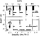 I. Vuorinen, M. Rajasilta & J. Salo in Oecologia, 1983, 59. [p.63, Fig.1]. I. Vuorinen, M. Rajasilta & J. Salo in Oecologia, 1983, 59. [p.63, Fig.1].
The density (ind./10 l) of nob-ovigerous females of Eurytemora hirundoides (= E affinis) at different depths at the Archipelago Sea on the SW coast of Finland in June August 1977 at 0900 h.
Nota: The distribution of ovigerous and non-ovigerous females followed a constant pattern through summer and early autumn. Non-ovigerous females were distributed throughout the water column, preferring the deeper parts. Ovigerous females were also abundant below 20 m but they almost totally avoided the surface layer above 20 m. The difference wqs statiscally significant.
When Eurytemora ovigerous and non-ovigerous females were presented for fish (Gasterosteus aculeatus, important planktivore predator) in an abundance corresponding to that found in nature (9 ind./750 ml), no selection between the two types was found. That was also the result when females and males were offered in densities much higher than natural (corresponding 133 ind./ l). When ovigerous and non-ovigerous females were presented in such high densities a significant preference was the result. (Table 1) |
 Issued from : D. Beyrend-Dur, S. Souissi, D. Devreker, G. Winkler & J.-S. Hwang in J. Plankton Res., 2009, 31 (7). [p.719, Table III]. Issued from : D. Beyrend-Dur, S. Souissi, D. Devreker, G. Winkler & J.-S. Hwang in J. Plankton Res., 2009, 31 (7). [p.719, Table III].
Values of the statistical parameters (R2, SSE and RMSE) fit to stage duration of E? affinis at 10°C and different salinities, represented in Fig.1
SSE: Error between the adjustment and the real distribution correspoding to the sum of square residuals. The percentage of variance explained by the gamma adjustment corresponds to R-suare (R2).The difference between the values predicted by the model and the values actually observed from the data modelled in the root mean squared error (RMSE).The closer the SSE and RMSE values are 0 and closer the R2 is to 1. the better the model fits. Once the parameters are known, the Median Development Time per stage (MDT) can be calculated (MATLAB software). whiçch computes the inverse of the cumulative GDF (according to the shape of the cumulative moulting distributions, it is fitted a gamma density function [see in Souissi & al., 1997] at any probability. In this study, the probability is 0.5, which corresponds to 50% of individuals having moulted. |
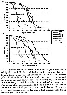
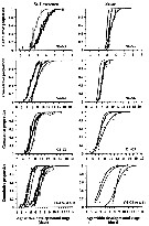 Issued from : D. Beyrend-Dur, S. Souissi, D. Devreker, G. Winkler & J.-S. Hwang in J. Plankton Res., 2009, 31 (7). [p.718, Fig. 1]. Issued from : D. Beyrend-Dur, S. Souissi, D. Devreker, G. Winkler & J.-S. Hwang in J. Plankton Res., 2009, 31 (7). [p.718, Fig. 1].
Cumulative proportion of individuals moulting from one group of stages to the next one as a functionol age within developmental stage(s) for both populations of E. affinis studied at 10°C.
Groups of stages were aggregated for naupliar stages (N1-N3 and N4-N6) and copepodid stages (C1-C3, C4-C5 M, and C4-C5 F).
Observed data from initial conditions in all experiments for both populations: St. Lawrence and the Seine estuary. |
 Issued from : D. Beyrend-Dur, S. Souissi, D. Devreker, G. Winkler & J.-S. Hwang in J. Plankton Res., 2009, 31 (7). [p.717, Table II]. Issued from : D. Beyrend-Dur, S. Souissi, D. Devreker, G. Winkler & J.-S. Hwang in J. Plankton Res., 2009, 31 (7). [p.717, Table II].
Mean (DT) and standard deviation (SD) of post-embryonic development time (days), and number of individuals (n) for seven different experimental conditions for both E. affinis populations.
Experimental conditions: ASL5, ASL15a, ASL15b, ASL25, ESS, ES15
, ES25. See Table 1: food supply and salinity.. |
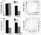
 Issued from : D. Beyrend-Dur, S. Souissi, D. Devreker, G. Winkler & J.-S. Hwang in J. Plankton Res., 2009, 31 (7). [p.721, Fig.4]. Issued from : D. Beyrend-Dur, S. Souissi, D. Devreker, G. Winkler & J.-S. Hwang in J. Plankton Res., 2009, 31 (7). [p.721, Fig.4].
Survival rate (%) during post embryonic-development and before maturation in response to dfifferent salinity (5, 15, 25) for E. affinis from the St. Lawrence salt-marshes (ASL) and the Seine estuary (ES).
Curves represent percentage of survival per developmental stage from N1 to C5. |
 Issued from : D. Beyrend-Dur, S. Souissi, D. Devreker, G. Winkler & J.-S. Hwang in J. Plankton Res., 2009, 31 (7). [p.722, Fig.5]. Issued from : D. Beyrend-Dur, S. Souissi, D. Devreker, G. Winkler & J.-S. Hwang in J. Plankton Res., 2009, 31 (7). [p.722, Fig.5].
Survival rate (%) of males (A) and females (B) in response to salinity (5, 15, 25) date and food (a and b) of two populations of E. affinis from the St. Lawrence (ASL) and the Seine estuary (ES) at 10°C. |
 Issued from : D. Beyrend-Dur, S. Souissi, D. Devreker, G. Winkler & J.-S. Hwang in J. Plankton Res., 2009, 31 (7). [p.723, TFig.6]. Issued from : D. Beyrend-Dur, S. Souissi, D. Devreker, G. Winkler & J.-S. Hwang in J. Plankton Res., 2009, 31 (7). [p.723, TFig.6].
Mean values of reproductive parameters of females observed in seven experimental conditions and for both E. affinis populations studied at 10°C: clutch size (eggs/ cluth) |
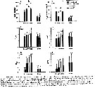
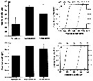 Issued from : A. Souissi, S. Souissi, D. Devreker & J.-S. Hwang in Ma. Biol., 2010, 157. [p.855, Fig. 2]. Issued from : A. Souissi, S. Souissi, D. Devreker & J.-S. Hwang in Ma. Biol., 2010, 157. [p.855, Fig. 2].
Prosome lengths (a) and widths (b) of both sexes of Eurytemora affinis adiuls (male and female) and the feminized male encountered in the 4th generation reared at 7°C. Individuals sampled in The Seine estuary.
Vertical bars represent standard deviation.
The cumulative probability distributions of prosome length (c) and prosome width (d) for males (continuous line) and females (discontinuoius lines) were obtained by bootstrap resampling (10,000 times). Vertical thin line and both thick arrows indicate the observed value of prosome length (c) and prosome width (d) for the feminized individuals. |
 Issued from : A. Souissi, S. Souissi, D. Devreker & J.-S. Hwang in Ma. Biol., 2010, 157. [p.856, Fig. 3]. Issued from : A. Souissi, S. Souissi, D. Devreker & J.-S. Hwang in Ma. Biol., 2010, 157. [p.856, Fig. 3].
Urosome lengths (a) and widths (b) of both sexes of Eurytemora affinis adults (male and female) and the feminizede males encountered in the 4th generation reared at 7°C. Individuals sampled in The Seine estuary.
verticval bars represent standard deviation.
The cumulative probability distributions of urosome length (c) and urosome width (d) for males (continuous line) and females (discontinuous lines) were obtained by bootstrap resampling (10,000 times).
Vertical thin line and both thick arrows indicate the observede value of urosome length (c) and urosome width (d) for the feminized individuals. |
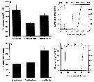
 Issued from : A. Souissi, S. Souissi, D. Devreker & J.-S. Hwang in Ma. Biol., 2010, 157. [p.858, Fig. 5]. Issued from : A. Souissi, S. Souissi, D. Devreker & J.-S. Hwang in Ma. Biol., 2010, 157. [p.858, Fig. 5].
Mean sizes of the 15th segment of the right A1 (a) and the P5 basipodite (b) of a normal male and a feminized mame nof Eurytemora affinis sampled in the Seine estuary and reared..
Vertical bars represent standard deviation.
The cumulative probability distributions of the 5th segment antennule's length (black curve) and width (gray curve) (c) and the P5 basipodite 's length (black curve) and width (gray curve) (d) for normal males were obtained by bootstrap resampli,g (10,000 times).
Vertical thin line and both thick arrows indicate the observed value of the length (black) and width (gray) of each secondary sexual character observed in feminized individuals. |
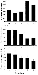 Issued from : A. Souissi, S. Souissi, D. Devreker & J.-S. Hwang in Ma. Biol., 2010, 157. [p.859, Fig. 7]. Issued from : A. Souissi, S. Souissi, D. Devreker & J.-S. Hwang in Ma. Biol., 2010, 157. [p.859, Fig. 7].
Total number of individuals produced per generation (a), sex ratio (abult females : adult males) (b) and clutch size (c) of Eurytemora affinis fsampled from The Seine estuary and cultured during 6 generations at 7°C.
The feminized males are observed at the 4th generation.
Vertical bars represent the standard deviation.
Nota: The appearnace of the intersex individuals in the culure at low temperature coincided with a decrease in food quality (Rhodomonas marina at its stationary phase). This induced a significant decrease in the mean clutch size and skewed sex ratio in favor of males. The reduction in food quality in addition to low temperature which induced slow development, are ssuspected to be responsible of the intersex individuals. This strssful situation seems to propagate to the following two generations at low temperature in contrast to the case of the experiment at higher temperature (20°C) where no intersex individual was observed |
 Issued from : P.H. Burkill & T.F. Kendall in Mar. Ecol. Prog. Ser., 1982, 7. [p.26, Fig.5]. Eurytemora affinis. Issued from : P.H. Burkill & T.F. Kendall in Mar. Ecol. Prog. Ser., 1982, 7. [p.26, Fig.5]. Eurytemora affinis.
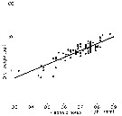
Length to weight relationship of different developmental stages in the Bristol Channel.
Equation: Log10 W= 2.088 (±0.119) L - 0.859 (±0.083).
Correlation coefficient (86 data points) 0.885.
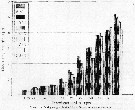
Dry weight (µg): 24th January: NVI = 0.36; CI = 0.51; CII = 0.78; CIII = 1.04; CIV = 2.215; CV = 3.15; CVI = 4.01. The 14 th May: CIII = 1.53; CIV = 2.60; CV = 3.82; CVI = 5.61. |
 Issued from : P.H. Burkill & T.F. Kendall in Mar. Ecol. Prog. Ser., 1982, 7. [p.25, Fig.4]. Eurytemora affinis. Issued from : P.H. Burkill & T.F. Kendall in Mar. Ecol. Prog. Ser., 1982, 7. [p.25, Fig.4]. Eurytemora affinis.
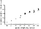
Size of different developmental stages during January (black circle), May (black square) and October (black triangle). Vertical bars: standard deviations.
Nota: Cephalothorax length showed a regular increases as the copepod developed and the variability of size generally increased with age. In the Bristol Channel there were no significant differences between the sizes found on different cruises (mean temperature and salinity, respectively: May 9.7-10.5 °C; 26.5-31.5 p. 1000; October 14.2-14.9 °C; 28.4-31.8 p.1000; Jan 5.8-7.2 °C; 25.4-31.1 p.1000. |
 Issued from : P.H. Burkill & T.F. Kendall in Mar. Ecol. Prog. Ser., 1982, 7. [p.26, Fig.6]. Eurytemora affinis. Issued from : P.H. Burkill & T.F. Kendall in Mar. Ecol. Prog. Ser., 1982, 7. [p.26, Fig.6]. Eurytemora affinis.
Variation in the proportion of the population moulting daily during January (circles), May (squares), and October (diamonds).
Nota: Development rates varied from stage to stage and from period. During each experimental period, the moulting rates of the different stages were inversely related to their ages.
Developmental rates proceeded faster when water temperatures were warmer. |
 Issued from : P.H. Burkill & T.F. Kendall in Mar. Ecol. Prog. Ser., 1982, 7. [Table 7]. Eurytemora affinis. Issued from : P.H. Burkill & T.F. Kendall in Mar. Ecol. Prog. Ser., 1982, 7. [Table 7]. Eurytemora affinis.
Comparison of development times of the copepod under simulated in-situ conditions and fed on algae (After Heinle & Flemer, 1975). |
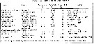
 Issued from : P.H. Burkill & T.F. Kendall in Mar. Ecol. Prog. Ser., 1982, 7. [p.26, Table 4]. Eurytemora affinis. Issued from : P.H. Burkill & T.F. Kendall in Mar. Ecol. Prog. Ser., 1982, 7. [p.26, Table 4]. Eurytemora affinis.
Standing stocks and daily production for different development stages in the Bristol Channel.
Nota: Standing stocks estimated from the weights of each stage and their abundance varied between 0.7 µg m-3 found on 2nd November and 22.2 µg m -3 on 14 th May. In January the biomass was 3.4 µg m-3.
Production rates varied seasonally, the lowest rate (0.051 µg m3 d-1 occurring in January. In May, values of 0.405 and 0.612 µg m-3 d-1 were estimated and rates of 0.064 and 0.076 µg m-3 d-1 were found in October and November, respectively.
Despite the fact that the younger stages moulted faster than older, the greater abundance and larger increase in weight per moult of older stages resulted in greater productivity of the CIII to CV stages in January. |
 Issued from : P.H. Burkill & T.F. Kendall in Mar. Ecol. Prog. Ser., 1982, 7. [p.27, Table 5]. Eurytemora affinis. Issued from : P.H. Burkill & T.F. Kendall in Mar. Ecol. Prog. Ser., 1982, 7. [p.27, Table 5]. Eurytemora affinis.
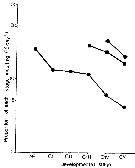
Daily production/biomasse values in the easten Bristol Channel.
Nota: The daily P/B values show a relationship with stage for each of the cruises.
The highest P/B ratio was 0.20 for copepodite III in May and lowest P/B was 0.01 for copepodite V in January
Population P/B, obtained by dividing the population production by standing stock varied from 0.03 in January to 0.13 in October. [See comparison with P/B quotients of some copepods in neritic regions and various temperatures. Table 6].x |
 Issued from : P.H. Burkill & T.F. Kendall in Mar. Ecol. Prog. Ser., 1982, 7. [p.28, Table 6]. Issued from : P.H. Burkill & T.F. Kendall in Mar. Ecol. Prog. Ser., 1982, 7. [p.28, Table 6].
Production/Biomasse quotients of some copepods in neritic regions. |
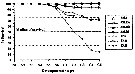
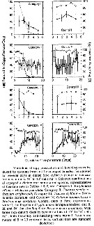
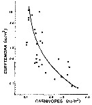 Issued from : P.H. Burkill & T.F. Kendall in Mar. Ecol. Prog. Ser., 1982, 7. [p.29, Fig.7]. Issued from : P.H. Burkill & T.F. Kendall in Mar. Ecol. Prog. Ser., 1982, 7. [p.29, Fig.7].
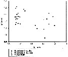
Eurytemora affinis from the Bristol Channel. Abundance as a function of carnivore abundance for separte hauls made in January, Mayb and October.
Line is fitted by eye.
Nota: predation is a factor influencing the Eurytemora affinis population [as all other copepods]. Several predator species were found in the plankton hauls carried out to estimate copepod abundance [the highter difficulty is to estimate the mortality rate by natural death and local predation for the different stages during the life cycle of the species]
There was an inverse relationship between the abundance of E. affinis and carnivore abundance, suggesting that predation influences the abundance of this copepod [as all other pelagic copepods; for instance in the Banyuls' Bay,. such a lot of chaetognathes leads to a drastic reduction in the copepods' population, but localement]. In January, the commonest planktonic group capable of taking E. affinis are mysids. In May, decapods such as Crangon crangon and another formed the largest component capable of consuming copepods.. Chaetognaths dominated the carnivorous component of the plankton in October. Also, fishes are predators. |
 Issued from : P.H. Burkill & T.F. Kendall in Mar. Ecol. Prog. Ser., 1982, 7. [p.25]. Issued from : P.H. Burkill & T.F. Kendall in Mar. Ecol. Prog. Ser., 1982, 7. [p.25].
Production estimation and Length-Weight relationship calculated for Eurytemora affinis from the Bristol Channel.
Nota: The mean abundance varied seasonally, ranging from 0.24 m-3 in november to 4.83 m-3 in May. There are considerable variation in abundance between tows, indicating that the copepod is not distributed evenly in the estuary.
In January, the population density had risen to 1.41 m-3.
It is pertinent that naupliar stages were found in January indicating that the population was reproducing; this contrast with oceanic species that typically over-winter at late copepodites stages, deferring reproduction until spring. |
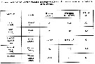
 Issued from : V. Escaravage & K. Soetaert in Cah. Biol. Mar., 1993, 34. [p.207, Table II]. Issued from : V. Escaravage & K. Soetaert in Cah. Biol. Mar., 1993, 34. [p.207, Table II].
Development stages mran duration (n : number of cultured copepods, d : mean stage duration, C.I. : confidence interval at 95%).
Sampling area in the lower estuarine part of the Schelde (Western Schelde estuary )collected from October 1989 to October 1990 in twelve stations from the mouth of the Westerschelde (Vlissingen) to Antwerp (limit of the saline intrusion). The copepods used in the cultures with a salinity always around 10 per 1000., the temperature ranges used in the cultures were chosen according to the cotrresponding field temperature in 1990 (April: 10°C, June: 17°C, March: 5°C); In June temperatures in cultures 14, 17 and 20°C; in March: 2, 5, 8°C. |
 Issued from : V. Escaravage & K. Soetaert in Cah. Biol. Mar., 1993, 34. [p.208, Table III]. Issued from : V. Escaravage & K. Soetaert in Cah. Biol. Mar., 1993, 34. [p.208, Table III].
a and b parameters characterizing the stage specific temperature dependent development rate (Development time = a ind.i x Tb ind.i. |
 Issued from : V. Escaravage & K. Soetaert in Cah. Biol. Mar., 1993, 34. [p.211, Table IV]. Issued from : V. Escaravage & K. Soetaert in Cah. Biol. Mar., 1993, 34. [p.211, Table IV].
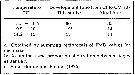
Development times obtained for E. affinis (from the Westerschelde, The netherlands) in laboratory cultures.
Dn : Naupliar development (hatch to CI), Dc : Copepodite development (CI to CV), Dt : total development = Dn + Dc (*: model adjusted on data provided by authors). |
 Issued from : V. Escaravage & K. Soetaert in Cah. Biol. Mar., 1993, 34. [p.212, Fig.7]. Issued from : V. Escaravage & K. Soetaert in Cah. Biol. Mar., 1993, 34. [p.212, Fig.7].
Comparison with other models found for E. affinis from hatching to adulthood. |
 Issued from : V. Escaravage & K. Soetaert in Cah. Biol. Mar., 1993, 34. [p.204]. Issued from : V. Escaravage & K. Soetaert in Cah. Biol. Mar., 1993, 34. [p.204].
Algorithm used after Rigler and Dowing (1984) method (modified by Polischuk, 1990) for estimation of the weight specific growth rates measurements and adult reproductive effort. |
 Issued from : V. Escaravage & K. Soetaert in Cah. Biol. Mar., 1993, 34. [p.209, Fig.4]. Issued from : V. Escaravage & K. Soetaert in Cah. Biol. Mar., 1993, 34. [p.209, Fig.4].
Production of eggs, spermatophores and somatic expressed as weight specific daily productions.
Results expressed in µg dry weight/ mg dry weight/day and compared with the mean daily somatic production measured from NII to CV.
The ratio between the reproductive and the somatic productions was not constant, it varied from 50 to 150% for the females but only from 40 to 60% for the males. The male production reached 40 to 90% of the female production. |
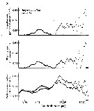
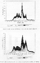 Issued from : V. Escaravage & K. Soetaert in Cah. Biol. Mar., 1993, 34. [p.210, Figs.5 and 6]. Issued from : V. Escaravage & K. Soetaert in Cah. Biol. Mar., 1993, 34. [p.210, Figs.5 and 6].
Fig.5 (above): Biomass of E. affinis (from Westerschelde estuary, The Netherlands) from October 1989 to October 19902.
Fig.6 (below): Production estimates obtained using the biomass showed above and the Polishchuk (1990) formula.
Nota: The in situ biomass evolution is characteristic for this species and can be divided in 3 phases: Winter emergence, Spring peak, Summer disappearance. Such pattern is supposed originated from a composition of internal dynamics (temperature controlled) and external control (predation, competition) (Bradley, 1975).
Combining this data set with the culture results (temperature controlled stage specific growth rates) one is able to estimate the production realized by the natural production (formulae in Ecological data methods).
The production realized by the adults (including the reproductive effort) represented 50% of the total production.
The daily production was estimated by 5 mg m3 day-1 and the annual integrated production by 1.6 mg. m3.
A global P/B of 33 year-1 was found for the whole population. |
 Issued from : V. Escaravage & K. Soetaert in Cah. Biol. Mar., 1993, 34. [p.213, Table V]. Issued from : V. Escaravage & K. Soetaert in Cah. Biol. Mar., 1993, 34. [p.213, Table V].
Biomass, Production, Productivity (P/B) ratios measured for E. affinis in other estuarine locations compared with the present study.Nota: Comparisons can be made between the present estimate of production and others obtained for the same species in comparable environments. Whereas the biomass differed in the different areas, the P/B values showed remarkably close values. This converged with the similarirties observede for the development rates obtained in cultures supplied either with natural particulate matter or with algal cultures. Both these observations underlinede the ethophysiologic plasticity of the estuarine species. |
 Issued from : V. Escaravage & K. Soetaert in Cah. Biol. Mar., 1993, 34. [p.208, Fig.3]. Issued from : V. Escaravage & K. Soetaert in Cah. Biol. Mar., 1993, 34. [p.208, Fig.3].
E; affinis from Westerschelde (The Netherlands) in culture.
Nota: A Log/Log weight length regression was calculated from individuals in the course of the culture experiments at different temperatures. No significative difference was found among cultures (different temperatures) or between the cultures and the field.
Following, all these data were pooled to establish a common weight length regression for the field and the culture : Log (W) = 2.441 x Log (L) - 6.095 (r2 = 0.97, p = <0.05). This relation was used to convert the molt lengths into the corresponding individual body dry weights from which were calculated the mean stage specific individual dry weights in the figure. |
 Issued from : C.B. Miller in Biological Oceanography 2004/2005, Blackwell Publishing. [p.139, Fig.7.6]. Issued from : C.B. Miller in Biological Oceanography 2004/2005, Blackwell Publishing. [p.139, Fig.7.6].
Exemple of selection by particle-feeding copepods from Chesapeake Bay. (a) The particle spectra before (dark circles) and after (open circles a day of feeding by female Eurytemora affinis. No particles of about 10 µm equivalent spherical diameter were removed and the filtering rate and ingestion rate spectra reflect that. (After Richman, Heinle & Huff, 1977). |
 Issued from : S. Ban, C. Burns, J. Castel, Y. Chaudron & al. in Mar. Ecol. Prog. Ser., 1997, 157. [p.289, Table 1]. Issued from : S. Ban, C. Burns, J. Castel, Y. Chaudron & al. in Mar. Ecol. Prog. Ser., 1997, 157. [p.289, Table 1].
Synopsis of feeding/reproduction experiments. A total of 17 diatom and 16 copepod species, representative of a variety of worldwide temperate and subarctic environments (E: estuarine, C: coastal ocean), were screened.
Data for fecundity and hatching success are average values measured at the start and end of the inciubations in a minimum of 3 replicate batches, showing the variation in time of the effects of diatoms on copepod reproduction.
Level of significance of the diatom effect between treatments and controls (e.g. non-diatom diets) in categories I to III was p < 0.01. No.. rank (for comparison with Table 2, p.290).
For the signification of the categories I to IV (fecundity vs. Hatching success vs. Duration of experiment days-1): See Eurytemora affinis, Calanus pacificus, Calanus finmarchicus, Temora stylifera.
List of the 12 marine or estuarine species studied (fresh water excluded. CR): Acartia clausi, A. grani, A. steueri, A. tonsa, Calanus finmarchicus, C. helgolandicus, C. pacificus, Centropages hamatus, C. typicus, Eurytemora affinis, Temora longicornis, T. stylifera. |
 Issued from : S. Ban, C. Burns, J. Castel, Y. Chaudron & al. in Mar. Ecol. Prog. Ser., 1997, 157. [p.288, Fig. 1]. Issued from : S. Ban, C. Burns, J. Castel, Y. Chaudron & al. in Mar. Ecol. Prog. Ser., 1997, 157. [p.288, Fig. 1].
Variations of egg production and hatching rates induced by diatoms ingested by copepod females maintained for several days in dense food cultures. Selected combinations of the data sets in Table 1 & 2. For categories in function of the duration of experiments (days).
See explanations in calanus finmarchicus (same Fig.1) |
 Issued from : S. Ban, C. Burns, J. Castel, Y. Chaudron & al. in Mar. Ecol. Prog. Ser., 1997, 157. [p.290, Table 2]. Issued from : S. Ban, C. Burns, J. Castel, Y. Chaudron & al. in Mar. Ecol. Prog. Ser., 1997, 157. [p.290, Table 2].
Combinations of copepod and non-diatom diets in controls in concentrations ranging from 104 to 105 cells ml-1. Data for fecundity and hatching success are average values measured at the start and end of incubation in a minimum of 3 replicate batches.
No 14: In Category I; No 34, 35: In Category III. |
| | | | Loc: | | | [non Argentina], Gulf of Mexico, Louisiana, Florida, Patuxent River estuary, Navesink River estuary, Petttaquamscutt estuary, Delaware Bay, Chesapeake Bay, Woods Hole, G. of Maine, Frenchman Bay (Maine), Northumberland Strait, Lake Erie, Canada (St. Laurent Estuary, Saquenay fjord), Labrador (Tessiarsuk fjord), Godthaab Fjord (W Greenland), Baltic (SW coast of Finland), Ireland, Tamar River estuary, Bristol Channel-Severn estuary, English Channel (Morlaix estuary), France (Etang de Berre, Gironde estuary, Charente estuary, le Croisic, Loire estuary, Seine estuary), Belgium (Scheldt estuary), Texel (Nertherlands), Schlei Fjord (Kiel Bay), Norway (estuaries), Svartatjønn basin, Barents Sea (estuaries), North Sea (estuaries), Elbe (estuary, Hamburg- Cuxhaven), Humber Estuary, Kiel Bay, E Baltic Sea, G. of Finland, G of Riga: Pärnu Bay; Öregrund Archipelago, Black Sea (Bay), Caspian Sea, Kuril Is., China Seas (Bohai Sea), Japan, Korea, Hokkaido (Lake Ohnuma), E Siberia, Strait of Georgia, British Columbia, Vancouver Is. (Nitinat Lake), Chehalis River estuary, San Francisco Bay & Estuary, California, SE Beaufort .Sea (in Darnis & al., 2008 (p.994, Table 1).
Type locality: Elbe River
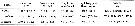
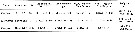
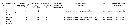
| | | | N: | 147 (? : species complex) | | | | Lg.: | | | (45) F: 1,6-1,4; M: 1,6-1,4; (145) F: 1,56; M: 1,15; (167) F: 1,73-1,19; M: 1,65-1,36; (564) F: 1,71-1,48; M: 1,65-1,4; (866) F: 1,28-1,4; M: 1,13-1,23; (1220) F: 0,8-1,9; M: 0,75-1,65; (1232) F: 1,0-1,56; M: 0,9-1,15; {F: 1,19-1,73; M: 1,13-1,65}
In culture (Katona, 1970): at 2°C: F= 1.778 mm ± 0.064; M= 1.498 mm ±0.044; at 20°C: F= 1.248 mm ±0.121; M= 1.154 mm ±0.016; between 10° and 20°C length was relatively constant and not significantly affected by different salinities from 8 to 35 p.1000.
After Kos (1976) the body length for E. hirundoides is 1.0-1.56 mm (females) and 0.9-1.15 mm (males). | | | | Rem.: | freshwater, brackish.
After Engel (1962) the presence of a re^producing population, represented by ovigerous females, suggests the possibility that E. affinis is established in Lake Erie.
After Heron & Damkaer (1976, Table 2) ratio anal somite/uropod (= caudal rami) 7/17; with metasomal wings in female, not in male.
Not all authors agree on the synonymy between this species and E. hirundoides.
Incomplete data.
For R.A. Engel (1962, p.252) this form is present in the Erie Lake
After Madéran & al. (2012) the species in the maximum turbidity zone, in the Charente estuary, were believed to reflect a higher carnivorus tendancy as a functional response to the strong decrease of phytoplankton availability; contrary to Acartia spp., unable to change their diet in the same way and was thus unable to colonize upstream areas.
After Alekseev & Souissi (2011, p.41, 51-52) in contrast to morphology-based taxonomy, recent molecular-genetic and cross-hybridization studies demontrated that E. affinis represents, in fact, a complex of sibling species with higfhly similar morphologies but isolated within the past million years (see Knowlton, 1993; Lee, 1999; 2000; Lee & Frost, 2002). Laboratory cross-hybridization studies between two divergent clades of E. affinis from Europe and North America indicated that hybrids in the second generation were sterile (Souissi S. pers. comm.). In E. affinis only a small proportion of adults in some local populations have setae on swimming legs with unclear segment-like divisions. They have mandible with more or less equal teeth; the outside tooth is not separated from neighboring teeth by a gap (vs a large outside tooth separated with a gap from other teeth in E. carolleeae). Female E. affinis (in contrast to E. carolleeae) has a genital somite with only small upper outgrowths (if present) which do not look like wings; the ratio between anterior and posterior parts in the genital somite is significantly less than 1.5 times (see Table 2). In P5 the tiny spine is much longer than width of the nearest distal spines and usually is more than 15% of the short distal spine length (see Table 4). Male E. affinis always has caudal rami with at least several spines on the dorsal surface. In P5 the left exopodal segment has a triangular shape outgrowth that decreases length/width proportion in this segment up to 1 or even less (see Table 3).
For Beyrend-Dur & al. (2009, p.713) the study of the life cycle of the populations from St. Lawrence (Canada) and from the Seine estuary (France) at three salinities (5, 15, 25) revealed differences in their salinity tolerance. Individuals from the Seine exhibited high mortality under the highest salinity than in the St. Lawrence population which tolerated a wider salinity range. At the lowest salinity, the development time of St. Lawrence individuals was longer than that of individuals from the Seine, suggesting that the Seine population were more adapted to low salinity. The clutch size and the longevity of St. Lawrence population exhibited a higher fitness relative to the Seine population. Such differences could be due to the genetic differences. The authors confirmed that a gamma density function is an appropriate fitting function for copepod development time. It can be integrated into individual-based models of copepod population dynamics.
The feeding mode after Barton & al. (2013, Table 1) is 'cruising' (See definition in Rem. Metridia pacifica). | | | Last update : 26/10/2020 | |
|
|
 Any use of this site for a publication will be mentioned with the following reference : Any use of this site for a publication will be mentioned with the following reference :
Razouls C., Desreumaux N., Kouwenberg J. and de Bovée F., 2005-2025. - Biodiversity of Marine Planktonic Copepods (morphology, geographical distribution and biological data). Sorbonne University, CNRS. Available at http://copepodes.obs-banyuls.fr/en [Accessed January 05, 2026] © copyright 2005-2025 Sorbonne University, CNRS
|
|
|
|


;)
;)
;)
;)
;)
;)
;)
;)
;)
;)
;)
;)
;)
;)
;)
;)
;)
;)
;)
;)
;)
;)
;)
;)
;)
;)
;)
;)
;)
;)
;)
;)
;)
;)
;)
;)
;)
;)
;)
;)
;)
;)
;)
;)
;)
;)
;)
;)
;)