|
|
 |
|
Calanoida ( Order ) |
|
|
|
Calanoidea ( Superfamily ) |
|
|
|
Calanidae ( Family ) |
|
|
|
Calanus ( Genus ) |
|
|
| |
Calanus helgolandicus (Claus, 1863) (F,M) | |
| | | | | | | Syn.: | Cetochilus septentrionalis: Grobben, 1881 (p.1, egg development); Cetochilus helgolandicus Claus, 1863 (p.171, figs.F,M);
Calanus finmarchicus : Giesbrecht, 1892 (part., p.89, figs.F); Farran, 1908 b (p.20, Rem.); Farran, 1926 (? part., p.227); 1929 (part., p.207, 212); Brian, 1914 a (p.134); Pesta, 1920 (p.493); Marques, 1966 (p.2); Mageed, 2006 (p.168, Table 4); Raymont & Krishnaswamy, 1960 (p.239, carbohydrate content);
no C. helgolandicus : Mori, 1937 (1964) (p.14, figs.F,M); Sewell, 1948 (p.550, 551, 544, 555, 565); C.B. Wilson, 1950 (p.178); Shih & Young,1995 (p.68);
Calanus : Harris & al., 1986 (p.845, Table 2, comparison pump vs. net) | | | | Ref.: | | | Sars, 1901 a (1903) (p.11, figs.F,M); Thompson & Scott, 1903 (p.232, 241); With, 1915 (p.12, Rem.); Früchtl, 1923 a (p.138, figs.F, Rem.); Sars, 1925 (p.6); Rose, 1929 (p.5); Wilson, 1932 a (p.25, figs.F,M); Rose, 1933 a (p.59, figs.F,M); Rees, 1949 (p.219, figs.F,M, juv.4,5); Brodsky, 1950 (1967) (p.99, figs.F,M); Farran & Vervoort, 1951 (n°32, p.3, Rem.); Marshall & Orr, 1952 (p.527, Table I: egg sizes); 1953 (p.1, fig.1: egg); Woodhead & Riley, 1957 (p.47, Rem.V, figs.); Jaschnov, 1957 (p.191, figs.); Furnestin, 1960 (p.167); Jaschnov, 1961 a (p.1317, biogeography); Brodsky, 1961 (p.15, figs.F,M); Gaudy, 1962 (p.93, 99, Rem.: p.100, Pl.I: juv., Tableau I: development); Giron-Reguer, 1963 (p.24); Harding, 1963 (p.81, karyotype); Grice, 1963 a (p.497, fig.F, Rem.); Vilela, 1965 (p.5); Mazza, 1967 (p.59, 62: clé juv.,F,M); Manwell & al., 1967 (p.145, biochimie); Matthews, 1967 a (p.159, Rev.); Vilela, 1968 (p.7); Koga, 1968 (p.16, fig.: egg); Corral Estrada, 1970 (p.62, figs.F, Rem.); Jillett, 1971 (p.29, Rem.); Marshall & Orr, 1972 (p.5, 8, 9, Rem.: p.53, fig.4); Brodsky, 1972 (1975) (p.9, 66, 81, 119, figs.); Vyshkvartzeva, 1972 (1975) (p.188, figs.); Williams, 1972 (p.53, figs.F, carte); Razouls, 1972 (p.91, 94, Tableau XXVI; Annexe: p.3, figs.F,M, Rem.); Bradford & Jillett, 1974 (p.6); Frost, 1974 (p.74, Rev.); Kos, 1976 (Vol.II, figs.F,M, Rem.; Fleminger & Hülsemann, 1977 (p.233, figs.F,M, geographical range-taxonomic divergence); Arnaud & al., 1980 (p.213, gut structure); Brodsky & al., 1983 (p.160, figs.F,M); van der Spoel & Heyman, 1983 (p.62, fig.79); Roe, 1984 (p.356); Sazhina, 1985 (p.23, figs.N); Grigg & al., 1987 (p.253, Rem. st.V); Fleminger & Hulsemann, 1987 (p.43: geographical mrophometric variation); Bradford, 1988 (p.76, Rem.); Nishida, 1989 (p.173, table 1, 2, 3: dorsal hump); Schnack, 1989 (p.137, tab.1, fig.6: Md); Bradford-Grieve, 1994 (p.31); Kouwenberg, 1994 (tab.1); Bucklin & al., 1995 (p.658); Harris, 1996 (p.95, 99); Kaartvedt, 1996 (p.145); Runge & Plourde, 1996 (p.171); Hure & Krsinic, 1998 (p.13, 99, 112); Lapernat, 1999 (p.10, 55); Lindeque & al., 1999 (p.91, Biomol.); Barthélémy, 1999 a (p.10, Fig.19); Bucklin & al., 1999 (p.239, molecular systematic); Bucklin & al., 2000 (p.1237, Rem.: analyse génétique moléculaire); Hill & al., 2001 (p.279, fig.2: phylogeny); Buttino & al., 2003 (p.469, fig. egg); G. Harding, 2004 (p.7, figs.F,M); Papadopoulos & al., 2005 (p.1353, phylogeography, molecular biology); Conway, 2006 (p.7: copepodite stages 1-6, Rem.); Unal & al., 2006 (p.1961, genetic analysis, phylogeography); Avancini & al., 2006 (p.59, Pl. 27, figs.F,M, Rem.); Ferrari & Dahms, 2007 (p.32, 34, Rem. N, p.62: copepodites); Vives & Shmeleva, 2007 (p.895, figs.F,M, Rem.); Blanco-Bercial & al., 2011 (p.103, Table 1, mol. Biol., phylogeny); Laakmann & al., 2013 (p.862, figs.1, 2, 3, 5, Table 1, 2, 3, mol. Biol.); Blanco-Bercial & al., 2014 (p.5: Rem.: problematic taxa); Bradford-Grieve & al., 2017 (p.17, Table 4: morphological data matrix character, Tale 6: GenBank, Table 19: setation of Mx2, Tablen 20: setation of Mx1, Table 21: setation of Mxp and P1., Fig.112. | 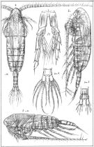 issued from : G.O. Sars in An Account of the Crustacea of Norway. Vol. IV. Copepoda Calanoida. Published by the Bergen Museum, 1903. [Pl. IIII]. Female & Male. Nota: Forehead like a ribbed vault in lateral view.
|
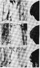 issued from : S.M. Marshall & A.P. Orr in The Biology of a Marine Copepod, Springer-Verlag (Ed.), 1972. [Fig.2]. Above drawings: Calanus finmarchicus Female (from North Sea): Coxa of the left P5; Proximal teeth of the coxa of the right P5; Forehead (lateral view). Middle drawings: Calanus finmarchicus Female (from Tromsö): Coxa of the left P5; Proximal teeth of the coxa of the right P5; Forehead (lateral view). Below drawings: Calanus helgolandicus Female (from North Sea): Coxa of the left P5; Proximal teeth of the coxa of the right P5; Forehead (lateral view), front slightly pointed. Nota: This species can be distinguished from C. finmarchicus by the following features: Coxa of P5 in stage V male and female is slightly convex internally. In male the endopod of the right P5 extends only a little beyond the distal margin of the 1st segment of the endopod. The head is slifhtly pointed. The eggs are rather larger (± 172 µm) than those of C. finmarchicus.
|
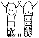 issued from K. Hulsemann in Invert. Taxon., 1994, 8. [p.1477, Fig.28, H]. Female: H, urosome (left: ventral); right: dorsal). Pore signature schematic by pooled samples (symbols are considerably larger than pores): Filled circle: 100 % presence; open circle: 95-99 % presence; triangle: 50-89 % presence. n = 400.
|
 issued from : R. Williams in Bull. mar. Ecol., 1972, 8. [p.57, Fig.3]. Female (from N Atlantic): Lateral view (i) and ventral view (ii) of three urosomes showing the variation in shape of the spermathecae and their lobed appearance.
|
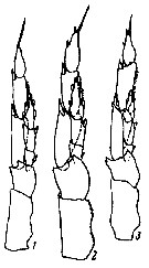
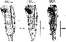 issued from : R. Williams in Bull. mar. Ecol., 1972, 8. [Plate XVII]. Female (from N Atlantic): lateral view of the urosome of the three species C. helgolandicus, C.finmarchicus and C. glacialis showing the differences in shape of their spemathecae. The edge of the operculum is easily seen in C. helgolandicus and C. finmarchicus.
|
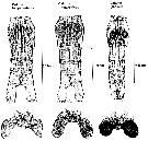 issued from : R. Williams in Bull. mar. Ecol., 1972, 8. [Plate XVIII, XIX]. Female (from N Atlantic): Above: Ventral view of the urosomes of the three species showing the obvious differences in shape of the spermathecae. The genital pore is in a more posterior position in C. glacialis than in the other two species. Below: A dorsal view of the spermathecae still attached to the basal plate. The spermatophore sac secretion which precedes the extrusion of the spermatozoa, is clearly seen in the spermathecae of C. finmarchicus. The lobed appearance of the spermathecal sacs of C. helgolandicus is also shown.
|
 issued from : N.V. Vyshkvartzeva in Issled. Fauny Moreï, 1972, 12 (20). [p.165, Fig.4, a, g]. Femele Md (masticatory edge, lateral): a, from North Sea; g, from Mediterranean Sea.
|
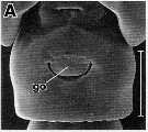 issued from : R.-M. Barthélémy in These Doct. Univ. Provence (Aix-Marseille I), 1999. [Fig.19, A]. Female (Gulf of Marseille: France): A, external ventral view genital double-somite. go = genital operculum. Scale bar: 0.100 mm.
|
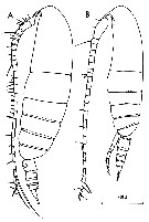 issued from : C. Razouls in Th. Doc. Etat Fac. Sc. Paris VI, 1972, Annexe. [Fig.20]. Female (from Banyuls, G. of Lion): A, habitus (lateral). Male: B, habitus (lateral).
|
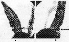
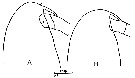 issued from : C. Razouls in Th. Doc. Etat Fac. Sc. Paris VI, 1972, Annexe. [Fig.21]. Female: Forehead comparison between C. helgolandicus A, from Banyuls (Gulf of Lion) and C. finmarchicus B, from isle of Cumbrae, loaned by S.M. Marshall (Marine Station Millport, Scotland). Nota; Forehead ogival in lateral view for C. helgolandicus (A) and perfectly rounded for C. finmarchicus (B).
|
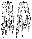 issued from : S.M. Marshall & A.P. Orr in The Biology of a Marine Copepod, Springer-Verlag (Ed.), 1972. [p. 14, Fig.4]. Comparison of P5 male from C. finmarchicus (d) and C. helgolandicus (e). Nota: Observe the lengths of endopodites and the inner edges of the coxa curvatures.
|
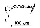 issued from : S.B. Schnack in Crustacean Issue, 1989,6. [p.143, 2]. 2, Calanus helgolandicus (from off NW Africa, upwelling region): cutting edge of Md.
|
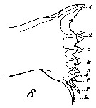 Issued from : W. Giesbrecht in Systematik und Faunistik der Pelagischen Copepoden des Golfes von Neapel und der angrenzenden Meeres-Abschnitte. - Fauna Flora Golf. Neapel, 1892, 19 , Atlas von 54 Tafeln. [Taf.7, Fig.8]. As Calanus finmarchicus. Female: 8, masticatory edge of Md (anterior view).
|
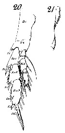 Issued from : W. Giesbrecht in Systematik und Faunistik der Pelagischen Copepoden des Golfes von Neapel und der angrenzenden Meeres-Abschnitte. - Fauna Flora Golf. Neapel, 1892, 19 , Atlas von 54 Tafeln. [Taf.8, Figs.20, 21]. As Calanus finmarchicus. Female: 20, P5 (anterior view); 21, inner margin of basipodite 1 (= coxa) of P5.
|
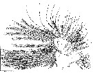 Issued from : W. Giesbrecht in Systematik und Faunistik der Pelagischen Copepoden des Golfes von Neapel und der angrenzenden Meeres-Abschnitte. - Fauna Flora Golf. Neapel, 1892, 19 , Atlas von 54 Tafeln. [Taf.7, Fig.13]. As Calanus finmarchicus. Female: 13, Mx1 §anterior view).
|
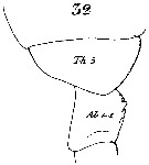 Issued from : W. Giesbrecht in Systematik und Faunistik der Pelagischen Copepoden des Golfes von Neapel und der angrenzenden Meeres-Abschnitte. - Fauna Flora Golf. Neapel, 1892, 19 , Atlas von 54 Tafeln. [Taf.7, Fig.32]. As Calanus finmarchicus. Female: 32, thoracic segment 5 (Th5) and genital segment (Ab 1-2 = genital double-somite).
|
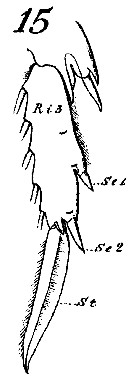 Issued from : W. Giesbrecht in Systematik und Faunistik der Pelagischen Copepoden des Golfes von Neapel und der angrenzenden Meeres-Abschnitte. - Fauna Flora Golf. Neapel, 1892, 19 , Atlas von 54 Tafeln. [Taf. 8, Fig.15]. As Calanus finmarchicus. Female: 15, exopodite 3 of P3 (anterior view).
|
 Issued from : W. Giesbrecht in Systematik und Faunistik der Pelagischen Copepoden des Golfes von Neapel und der angrenzenden Meeres-Abschnitte. - Fauna Flora Golf. Neapel, 1892, 19 , Atlas von 54 Tafeln. [Taf. 8, Fig.3]. As Calanus finmarchicus. Female: 3, A1, segments 1 to 17 (ventral view).
|
 Issued from : W. Giesbrecht in Systematik und Faunistik der Pelagischen Copepoden des Golfes von Neapel und der angrenzenden Meeres-Abschnitte. - Fauna Flora Golf. Neapel, 1892, 19 , Atlas von 54 Tafeln. [Taf. 8, Fig.3]. As Calanus finmarchicus. Female: 3, A1, segments 17 to 25 (ventral view).
|
 issued from : R. Gaudy in Rev. Trav. St. Mar. End., Bull. 27 (42). [p.125, Tableau I]. Identification of copepodids stages Calanus helgolandicus. A: Stage; B: number of swimming legs; C: number of thoracic segments; D: number of abdominal segments; E, Size.
|
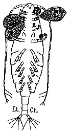 issued from : G. Trégouboff & M. Rose in Manuel de planctonologie méditerranéenne, 1957, CNRS, Paris. [Pl. 125]. Calanus helgolandicus female scematic ventral view (from Medirrranean Sea): Outer parasit Ellobiopsis chattoni fixed on copepod's appendages.
|
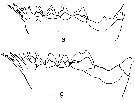
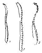 issued from : K.A. Brodsky in Zool. Zh., 1959, 38, 10. [p.1541, Fig.3]. Comparison of coxopodite inner edge of P5 female for Calanus glacialis (1), Calanus finmarchicus (2) and Calanus helgolandicus (3). Nota: Calanus glacialis : Dentate plate on coxopodite has very short, blunt teeth and is sligh curved in central position. Teeth are close together, without spaces, numbering 30-34. Calanus finmarchicus : Dentate plate on coxopodite has short, blunt teeth, with small spacings. Teeth-line not curved. Number of teeth 29-30. Calanus helgolandicus : Dentate plate on coxopodite very characteristic; teeth have more or less parallel edges, are relatively small, strongly marked curve in middle of line; distal part of plate has closely set, elongated teeth; spaces between teeth only in central part of line, teeth here are rounded, not flat. Number of teeth 28 (according to Jaschnov most specimens from the North Sea had 28-33 teeth).
|
 issued from : K.A. Brodsky in Zool. Zh., 1959, 38, 10. [p.1542, Fig.4]. Comparison of left leg of P5 for Calanus glacialis (1), Calanus finmarchicus (2) and Calanus helgolandicus (3). Nota: Calanus glacialis : In segments of exopodite of left leg, the relation of width of 1st and 2nd segments to length of corresponding segments is 1 : 3. Left endopodite reaches almost half the length of the 2nd segment of the exopodite of the same leg. Calanus finmarchicus : Relation of width to length of 1st and 2nd segments of exopodite of left leg is 1 : 2.5. Left endopodite extends beyond middle of 2nd segment of exopodite. Calanus helgolandicus : Relation od width to length of 1st and 2nd segments of exopodite of left leg is 1 : 2.5. left endopodite reaches distal limit of first third of 2nd segment of exopodite of same leg.
|
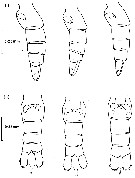
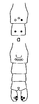 Issued from : A. Fleminger & K. Hulsemann in Mar. Biol., 1977, 40. [p.243, Fig.6 a]. Pore signature patterns of female urosome (ventral view shown below, dorsal view of genital segment and segment 2 (above). Specimens (n = 50) from North Atlantic localities. Filled circles: integumental pore present in all specimens examined; open circles: pore present in from 90 to 99% of specimens examined. Symbols used to indicate pores are not proportionate to actual pore size (latter range from 1 to 3 µm in diameter). Nota: The distribution of integumental organs on the urosome of adult females was determined in specimens selected at random from samples representing a variety of localities within the North Atlantic distribution. Calanus helgolandicus is most distinctive in lacking the 2 pairs of pores found in C. finmarchicus and C. glacialis on the ventral side of urosomal segments 2 and 3 and in having only 3 pores on the dorsal side of the genital segment.
|
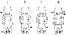 Issued from : A. Fleminger & K. Hulsemann in Mar. Biol., 1977, 40. [p.244, Fig.7]. Calanus helgolandicus Female: Integumental gland on ventral side of urosomal segments sites occupied in samples from (a) Western North Atlantic shelf and slope water (N = 19, MARMAP Cruise); (b) Mid-North Atlantic (N = 20); (c) Eastern North Atlantic off Europe (N = 20); (d) Eastern North Atlantic off Africa (N = 20). Filled circles: pore present in all specimens of sample; open circles: pore present in 90 to 99% of specimens; triangles: pore present in 20 to 49% of specimens; dots: pore present in 1 to 19% of specimens. Actual number of specimens with pore at indicated site is shown in arabic numerals when less than 100%. Symbols used to indicate pores are not proportionate to actual pore size (latter range from 1 to 3 µm in diameter). Nota: If the geographical variation we observed in the urosome pore signature of females proves to be real, it would demonstrate the lack of panmixis and the presence of two or more semi-independent populations in the North Atlantic Ocean. It is not unlikely that this species was temporarily eliminated from the North Atlantic during Pleistocene glaciations. The population in the Mediterranean Sea probably served as the promary reservoir for C. helgolandicus replenishing the North Atlantic when conditions were favorable, while otherwise regularly contributing to the specie's North Atlantic gene pool.At present, the Mediterranean sub-surface outfall undoubtedly carries C. helgolandicus into the North Atlantic just as Atlantic surface waters provide a conduit for gene flow in the opposite direction.
|
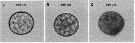 Issued from : C. Lauritano, Y. Carotenuto, G. Procaccini, J.T. Turner & A. Ianora in Harmful Algae, 2013, 28. [p.27, Fig.3] Egg images. Confocal microscope images of eggs spawned by females fed on the dinoflagellate Prorocentrum minimum (A) for one day or Karenia brevis for one (B) or three days (C). Nota: After one day of feeding on Karenia brevis, eggs collected soon after spawning were morphologically similar to the control (A), even if the cytoplasm and nuclei were not clearly defined (B). Conversely, after 3 days of feeding, eggs exhibited altered membrane cell morphology and apoptotic features such as granulation and degeneration of the cytoplasm matrix (C), whereas control eggs were identical to the first day. Ingestion of Kerenia brevis causes adverse effects on copepods, included alterations in copepod swimming and photobehavior, reduction in egg production and egg viability, and in some cases, reduced survival. In the study, although none of the females died, expression patterns of selevted genes involved in stress responses, detoxification mechanisms and apoptosis regulation were significantly affected.
|
 Issued from : P.M.J. Woodhead & J.D. Riley in J. Cons. int. Expl. Mer, 1957, 23. [p.48, Fig.1]. Side view of the urosome in potential male (a) and female (b) stage-V copepodites of Calanus helgolandicus from the western part of the English Channel in June 1950. Nota: the two types are distinguished by the degree of curvature of the ventral surface of the first (proximal) urosome segment (indicated by arrows).
|
 Issued from : P.M.J. Woodhead & J.D. Riley in J. Cons. int. Expl. Mer, 1957, 23. [p.50, Table 1]. The two size-groups in stage-V copepodites of Calanus helgolandicus separating the males from from females.
|
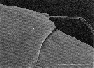 Issued from : J.M. Bradford-Grieve, L. Blanco-Bercial & G.A. Boxshall in Zootaxa, 2017, 4229. [p.18, Fig. 4]. Scanning electron micrograph of female antennule ancestral segments IV and V of Calanus helgolandicus. White arrow indicates dorsal hair sensillum on the dorsal surface. Scale bar = 50 µm. Nota: On the antennules of female, hair sensilla were difficult to see and were examined using a bench top scanning electron microscope (SEM). Character used in cladistic analysis and as outgroup in molecular phylogenetic analysis for other calanoid families. The authors use the term ''hair sensillum'' because there is no adjacent pore to an integumental gland (see in Fleminger, 1973).
|
 Issued from M. Rose in Résult. Camp. scient. Prince Albert I, 1929, 78, p.6. Remarques concernant Calanus finmarchicus et Calanus helgolandicus. See differences between the two species after S.M. Marshall & A.P. Orr, 1972 (p.7-8, fig.2)
| | | | | Compl. Ref.: | | | Pearson, 1906 (p.4, Rem.); Chatton, 1920 (p.16: Rem.; p.17); Rose, 1925 (p.151); Wilson, 1932 (p.21); 1942 a (part., p.172); Sewell, 1948 (p.347); C.B. Wilson, 1950 (part., p.178, non Pacif. stations); Duran, 1955 (p.52); Marshall & Orr, 1956 (p.587, feeding, young stages); Woodhead & Riley, 1957 (p.47; Jaschnov, 1958 (p.838, fig.2); Woodhead & Riley, 1959 (p.465, stage 5 M & F, sex ratio); Corner, 1961 (p.5, Table I: feeding, assimilation, filtering rate, oxygen consumption); Carlisle & Pitman, 1961 (p.827, neurosecretion-diapause); V.N. Greze, 1963 a (tabl.2); Zeiss, 1963 (p.110, respiration rates); Giron-Reguer, 1963 (p.24); Cowey & Corner, 1963 (p.495, amino acid composition, respiration); Rice, 1964 (p.163, hydrostatic pressure effects); Mazza, 1964 (p.293, weight); Grice & Hulsemann, 1965 (p.223, 225: Rem.); Linford, 1965 (p.16, Rem.: p.25, lipid content); Bodo & al., 1965 (p.219, annual cycle); Vucetic, 1965 (p.419, annual variations); 1965a (p.425, sex ratio, life history); 1965 b (p.431, annual variation length-weight); 1966 (p.1-91, life history); Mazza, 1966 (p.69); Ehrhardt, 1967 (p.737, geographic distribution), Rem.); Manwell & al., 1967 (p.145, electrophoresis-enzymes); Corner & Newell, 1967 (p.113, nitrogen excretion); Glover, 1967 (p.189, fig.5, annual abundance); Corner & Cowey, 1968 (p.393, Table 5, 8, aminoacid composition, assimilation); Robertson, 1968 (p.185, Text-Fig.5, abundance); Macdonald & al., 1972 (p.213, fig.4, hydrostatic pressure effect); Evans, 1968 (p.11); Vinogradov, 1968 (1970) (p.94, 268, 269); Keegan, 1969 (p.137, abundance); Mullin, 1969 (p.308, Table I: estimates of production); Champalbert, 1969 a (p.624); Richman & Rogers, 1969 (p.701, feeding vs. growing diatom); Singarajah, 1969 (p.171, Table I, II, behaviour); Butler & al., 1969 (p.977, nutrition/metabolism); 1970 (p.525, Rem.: p.529); Kovalev, 1969 a (p.146); 1970 a (p.87, Tableau 1, 2, comparison hyponeustonic & planctonic forms); Jaschnov, 1970 (p.204, chart); Paffenhöfer, 1970 (p.346, cultivation); Paffenhöfer & Sreickland, 1970 (p.97, feeding); Mullin & Brooks, 1970 (p.89, production); Shih & al., 1971 (p.36); Lee R.F. & al., 1971 (p.99, lipids); Lincoln, 1971 (p.677, fig.2, 3, hydrostatic pressure & illumination effects); Bainbridge & Forsyth, 1972 (p.21, Table I: indictor species); Roe, 1972 (p.277, tabl.1, 2); 1972 a (p.316); Corkett, 1972 (p.171, eggs: development rate); Corner & al., 1972 (p.847, feeding, excretion); Razouls S., 1972 b (p.2, respiration); Nival & al., 1972 (p.63, respiration); Gaudy, 1972 (p.175, 218, figs.25-27, annual cycle, Rem.: p.223-4); Eriksson, 1973 (p.37, fig.6, 7, 9, annual cycle); 1973 b (p.113, 118); Guglielmo, 1973 (p.399); Champalbert & al., 1973 (p.529, CHN composition); P. Nival & S. Nival, 1973 (p.135, mouth parts, grazing); Nival & al., 1973 (p.123, respiration); Nival & al., 1974 (p.231, respiration & excretion); S. Razouls, 1974 (147, oxygen rate); Corner & al., 1974 (p.319, feeding, nauplii diet); Corral Estrada & Pereiro Muñoz, 1974 (tab.I); Vives & al., 1975 (p.35, tab.II, III, IV); Fernandez, 1975 (p.1, fig.5, 6, 7, 8, 9, 10, 22, metabolism/lux); Corner & al., 1976 (p.345, animal diet, metabolism); Corner & al., 1976 (p.121, hydrocarbon effects); Paffenhöfer, 1976 (p.49, feeding behaviour); Deevey & Brooks, 1977 (p.256, Table 2, Station "S"); Sargent & al., 1977 (p.525, grazing); Greve, 1977 (p.83, feeding); Harris & al., 1977 (p.187, polluant effect); Colebrook, 1978 (tab.1); Fernandez, 1978 (p.97, metabolism/food, Rem.: Table 19); Comaschi Scaramuzza, 1978 (p.16); O'Hara & al., 1979 (p.331, sex hormone); Spooner & Corkett, 1979 (p.197, feeding rates vs oil effects); Andronov & Maigret, 1980 (p.65, Table 1, 2, 3); Hallberg & Hirche, 1980 (p.283, gut ultrastructure, enzymes); Hirche, 1981 (p.174, enzymes); Collins & Williams, 1981 (p.273, monthly distribution-salinity); Brenning, 1981 (p.1, spatial distribution, T-S diagram, Rem.); Kovalev & Shmeleva, 1982 (p.82); Vives, 1982 (p.290); Williams & Robins, 1982 (p.271, preservation modes vs. length, weight, nitrogen & carbon); Borgmann, 1982 (p.668, size/production); Castel & Courties, 1982 (p.417, Table II, spatial distribution); Hirche, 1983 (p.281); Rivière, 1983 (p.19, enzymes); Tremblay & Anderson, 1984 (p.4); Bottrell & Robins, 1984 (p.259, size/weight/Carbon & Nitrogen); Scotto di Carlo & al., 1984 (p.1042); Alvarez-Marques, 1984 (p.110, annual abundance, figs.F,M); Petipa & Ostravskaya, 1984 (p.631, energy expenditure), Baars & Fransz, 1984 (p.120, Table 1, grazing); Baars & Oosterhuis, 1984 (p.97, diurnal feeding rhythms); Mayzaud O. & al., 1984 (p.15, feeding/enzyme); Prahl & al., 1984 (p.317, assimilation); Hirche, 1984 (p.233, seasonal distribution); Boucher, 1984 (p.469, spatial distribution/hydrological front); Regner, 1985 (p.11, Rem.: p.20); Brenning, 1985 a (p.3, Table 2, fig.9); Jansa, 1985 (p.108, Tabl.I, , II, III, IV, V); Williams & Collins, 1985 (p.28); Nott & al., 1985 (p.271, gut histology, fecal pellet); Neal & al., 1986 (p.1, feeding); Diel & Klein Breteler, 1986 (p.85, growth, development rate); Robinson & Hunt, 1986 (p.791, Table 1, 2, fig.2); Harris & Malej, 1986 (p.75, vertical migration vs. ammonium excretion); Robinson & al., 1986 (p.201, seasonal & spatial distributions); Gill & Poulet, 1986 (p.193, appendage activity); Brylinski, 1986 (p.457, spatial variations); Quisthoudt & al., 1987 (p.995, spatial distribution); Comaschi Scaramuzza, 1987 (tab.1); Ibanez & Boucher, 1987 (p.205, Tableau, fig.5, 7, hydrological fronts); Boucher & al., 1987 (p.133, spatial distribution/physical structure); Williams R. & al., 1987 (p.247, vertical distribution); Gill & Harris, 1987 (p.785, feeding behaviour); Grigg & al., 1987 (p.253, biometry, development); Poulet & Gill, 1988 (p.259, feeding behaviour); McLaren & al., 1988 (p.275, DNA content, development rate: egg-nauplius); Gorsky & al., 1988 (p.133, Table I, C-N composition); Lozano Soldevilla & al., 1988 (p.57); Roy & al., 1989 (p.145, feeding); Giguère & al., 1989 (p.522, Table 1, formaldehyde preservation); Kattner & Krause, 1989 (p.261, Table 3, 4, 5, lipids); Poulet & al., 1989 (p.1325, Table 2, 3: vitamin content); Kouwenberg & Razouls, 1990 (p.23, climatic change); Krsinic, 1990 (p.337, Table I-II, vertical distribution); Fransz & al., 1991 (p.5 & suiv.); Hay & al., 1991 (p.1453, Table 2, 5); Scotto di Carlo & al., 1991 (p.271); Green & al., 1992 (p.1631, Nauplii-fecal pellets); Bautista & Harris, 1992 (p.41, ingestion rate, gut contents); Seguin & al., 1993 (p.23, Table 2: abundance, %); ); Fromentin & al., 1993 (p.285, Ligurian transect abundance); Morales C.E. & al., 1993 (p.185); Kouwenberg, 1993 (p.215, fig.3, seasonal abundance); 1993 a (p.281, fig.3, 4, sex ratio); Guerin-Ancey & David, 1993 (p.119, table 1, biovolume, vertical distribution); Hays & al., 1994 (tab.1); Harris, 1994 (p.431, ingestion & egestion); Poulet & al., 1994 (p.79, eggs); 1995 (p.85, eggs, Nauplii); Krause & al., 1995 (p.81, Rem.: p.128); Laabir & al., 1995 (p.1125, egg production vs. algal concentrations, fecal pellets); Guisande & Harris, 1995 (p.476, eggs, hatching success, naupliar survival); Southward & al., 1995 (p.127, fig.2, 3, 8, 13, distribution-abundance vs. time); Pond & al., 1995 (p.75, gut-pH); Weikert, 1995 (p.218, Rem.); Fernandez de Puelles & al., 1996 (p.97, occurrence: p.101); Fromentin & Planque, 1996 (p.101, spatial & temporal pattern); 1996a (p.111, distribution vs. NAO); Stöhr & al., 1996 (p.457, abundance); Zauke & al., 1996 (p.141, Table 7, metal bioaccumulation); Siokou-Frangou, 1997 (tab.1); Ban S, Burns C. & al., 1997 (p.287, Table1, 2, fig.3, feeding, reproduction); Gilabert & Moreno, 1998 (tab.1, 2); Reid & Hunt, 1998 (p.310, figs.2, 3, Rem.); Kouwenberg, 1998 (p.203, seasonal variation, fig.3: global change); Beare & McKenzie, 1999 (p.241, fig.6, 7); Miralto & al., 1999 (p.173, Rem.: p.174, egg production vs. diatoms effect of inhibition); Seridji & Hafferssas, 2000 (tab.1); Kang H-K & Poulet, 2000 (p.241, diet vs. reproduction); Kang H-K & al., 2000 (p.2171, diets vs reproduction); Ku Kang & al., 2000 (p.2171, reproduction vs diets); Moraitou-Apostolopoulou & al., 2000 (tab.I); d'Elbée, 2001 (tabl. 1); Lapernat & Razouls, 2001 (tab.1); Holmes, 2001 (p.36, Rem.); Fransz & Gonzalez, 2001 (p.255, tab.1); Weikert & al., 2001 (p.227, tab.4, fig.6, 8, 9, Rem.); Bressan & Moro, 2002 (tab.2); Zerouali & Melhaoui, 2002 (p.91, Tableau I); Beaugrand & al., 2002 (p.1692); Beaugrand & al., 2002 (p.179, figs.5, 6); Lindley & Reid, 2002 (p.153, abundance veriation); Reid & al., 2003 (p.260, figs.3,5); Titelman & Kiørboe, 2003 a (p.137, nauplius behaviour); Gaudy & al., 2003 (p.357, tab.1); Kane, 2003 (p.151); Morgado & al., 2003 (p.S205, abundance vs. ebbs and floods in estuary); Vukanic, 2003 (p.139, tab.1); Bode & al., 2003 (p.85, Table 1, abundance); Vieira & al., 2003 (p.S163, Table 2, abundance); Wexels Riser & al., 2003 (p.301, grazing vs. faecal pellets, toxins algae); Niehoff & Runge, 2003 (p.1581, gonad development, egg production predicted); Poulet & al., 2003 (p.889, Nauplius vs. food toxic or not); Romano & al., 2003 (p.3487, embryo vs. diatom toxicity); Lindeque & al., 2004 (p.121, fig.2); Fernandez de Puelles & al., 2004 (p.654, fig.7); Vinogradov & Musaeva, 2004 (p.503, Rem: p.512); CPR, 2004 (p.50, fig.139); Lopez-Urrutia & al., 2004 (p.303, clearance rate, predation); Koppelmann & al., 2004 (p.1, Rem.); Vallet & Dauvin, 2004 (p.539, tab.2); Miller C.B., 2005 (p.221, Rem., vs. Gulf Stream, CPR time series vs. NAO, fig. 16.11, 16.12); Veistheim & al., 2005 (p.382, tab.1, 2, fig.1); Souissi & al., 2005 (p.161); Siokou-Frangou & al., 2005 (p.160); Molinero & al., 2005 (p.156); Yebra & al., 2005 (p.1367, growth: C5-C6); Jonasdottir & al., 2005 (p.1239, egg production & hatching success); Bonnet & al., 2005 (pp.1-53, tab.2., overview in European waters); Queiroga & al., 2005 (p.195, table 1); Hays & al., 2005 (p.337, fig.1, climate change); Rawlinson & al., 2005 (p.205, tidal exchange); lindeque & al., 2006 (p.221); Albaina & Irigoien, 2006 (p.413, effect of the parasite Ellobiopsis); Isari & al., 2006 (p.241, tab.II); Marques & al., 2006 (p.297, tab.III); Zervoudaki & al., 2006 (p.149, Table I); Jansen & al., 2006 (p.102, nutrition); Varela & al., 2006 (p.272, Table 3, oil spill effects); Ceballos & Alvarez-Marqués, 2006 (p.1, dynamic of population); 2006a (p.189, reproduction); Poulet, Wichard & al., 2006 (p.129, egg production vs diatoms); Sommer F. & al., 2006 (p.167, astaxanthin vs. vertical distribution); Koppelmann & Weikert, 2007 (p.266: tab.3); Kouwenberg & Lantoine, 2007 (p.239: UV-B effects); Cook & al., 2007 (p.757, Naupliar development times); Helaouët & Beaugrand, 2007 (p.147, climate change effects); Fernandez de Puelles & al., 2007 (p.338, 348); Albaina & Irigoien, 2007 (p.433, Tab.1); Valdés & al., 2007 (p.103: tab.1); Poulet & al., 2007 (p.415, abnormal reproduction); Busatto, 2007 (p.26, Tab.3); Ferrari & Dahms, 2007 (p.63, Rem.); Fileman & al., 2007 (p. 70, grazing); Khelifi-Touhami & al., 2007 (p.327, Table 1); Vincent & al., 2007 (p.295, Table 1, 3, 6, 7, fig.2, nitrogen transfert); Hirst & al., 2007 (p.189, seasonal dynamics, mortality rates); Fontana & al., 2007 (p.1810, fig.3: egg hatching success, teratogenic effects vs. diatom toxicity; fig.4: nauplii malformation); Iversen & Poulsen, 2007 (p.79, coprophagy, clearance, Ingestion, coprorhexy); Cabal & al., 2008 (289, Table 1); Gaard & al., 2008 (p.59, Table 1, N Mid-Atlantic Ridge); Wichard & al., 2008 (p.30, reproduction); Molinero & al., 2008 (p.271, fig.4); Brylinski, 2009 (p.253, Tab.1); Labat & al., 2009 (p.1746, Table 2); Licandro & Icardi, 2009 (p.17, Table 4); Park & Ferrari, 2009 (p.143, fig.2, biogeography); Mackas & Beaugrand, 2010 (p.296, figs.11, 12); Bonnet & al., 2010 (p.725, Rem.: predation by Sagitta setosa); Fileman & al., 2010 (p.709, Rem.: feeding); Eloire & al., 2010 (p.657, Table II, temporal variability); Mazzocchi & Di Capua, 2010 (p.424); Vogedes & al., 2010 (p.1471, lipid sac area vs lipid content); Ianora & Miralto, 2010 (p.493, Fig.3: daily mean egg production rates and egg viability vs diatom diets); Mazzocchi & al., 2011 (p.1163, fig.6, long-term time-series 1984-2006); Fileman & al., 2011 (p.403, abundance vs bloom condition); Nowaczyk & al., 2011 (p.2159, Table 2); S.C. Marques & al., 2011 (p.59, Table 1); McGinty & al., 2011 (p.120, seasonal abundance vs N Atlantic zones); Jonasdottir & Koski, 2011 (p.85, vertical distribution, production); Bicknell & al., 2011 (p.1794, Table 1, 2, effects of formalin preservation); Isari & al., 2011 (p.51, Table 2, abundance vs distribution); Zervoudaki & al., 2011 (p.45, fig. 3 as Calanus spp, Table 3, abundance, egg production: Turkish Straits); Castellani & al., 2011 (p.104: Rem.); Van Ginderdeuren & al., 2012 (p.3, Table 1, Rem.: p.10); Lauritano & al., 2011a (p. 1, feeding vs toxicity, molecular expression); Lauritano & al., 2012 (p.22, Table 1, 2, gene/polluants); Zizah & al., 2012 (p.79, Tableau I, Rem.: p.86, 89); Miloslavic & al., 2012 (p.165, Table 2, transect distribution); Aubry & al., 2012 (p.125, table 3, fig. 6, 8 a, b, interannual variation); Salah S. & al., 2012 (p.155, Tableau 1, Rem.); Carotenuto & al., 2012 (p.46, population dynamics, egg production vs diets, cultivation); Lauritano & al., 2012 (p.1, genetic expression vs stress); Mayor & al., 2012 (p.258, fig.2, 3, hatching vs temperature & CO2 effects); McGinty & al., 2012 (p.122, time series abundance); Turner & al., 2012 (p.63, toxic dinoflagellate effects); Mazzocchi & al., 2012 (p.135, annual abundance 1984-2006); Madurell & al., 2012 (p.1078, submarine pump); Bode & al., 2012 (p.108, spatial distribution vs time-series, % biomass); Alvarez-Fernandez & al., 2012 (p.21, Rem.: Table 1); Møller & al., 2012 (p.211, development time vs temperature & food); Gusmao & al., 2013 (p.279, Table 4, sex ratio); Belmonte & al., 2013 (p.222, Table 2, abundance vs stations); Helaouët & al., 2013 (p.1, long-term changes abundance; 1958-2008); Lauritano & al., 2013 (p.23, dinoflagellate toxic effect vs. genes); Sobrinho-Gonçalves & al., 2013 (p.713, Table 2, fig.8, seasonal abundance vs environmental conditions); Gerdts & al., 2013 (p.757, Table 1: microbiome vs copepod); Breckels & al., 2013 (p.2486, swimming behavior vs algal metabolites); Cole & al., 2013 (p.6646, microplastic ingestion); Peijnenburg & Goetze, 2013 (p.2765, genetic data); Kürten & al., 2013 (p.167, Table 1, C:N, fatty acid); Maar & al., 2013 (p.24, spatial distribution, long-term changes); Lidvanov & al., 2013 (p.290, Table 2, % composition); Barton & al., 2013 (p.522, Table 1: metabolism, diapause, population dynamic, feeding mode, biogeo); Siokou & al., 2013 (p.1313, fig.5, 7, biomass, vertical distribution); Bonnet & al., 2013 (p.1, overview: ecology in European waters); Zaafa & al., 2014 (p.67, Table I, occurrence); Fernandez de Puelles & al., 2014 (p.82, Table 3, seasonal abundance); Mazzocchi & al., 2014 (p.64, Table 3, 4, 5, spatial & seasonal composition %); Zakaria & al., 2016 (p.1, Table 1); Benedetti & al., 2016 (p.159, Table I, fig.1, functional characters); Baumgartner & Tarrant, 2017 (p.387, Table 1, diapause); El Arraj & al., 2017 (p.272, table 1, Rem.: p.281); Benedetti & al., 2018 (p.1, Fig.2: ecological functional group); Record & al., 2018 (p.2238, Table 1: diapause); Richirt & al., 2019 (p.3, Table 1, fig.2, 3, 4, 5, abundance changes vs. years 1998-2014, table 2: diversity index); Belmonte, 2018 (p.273, Table I: Italian zones); Chaouadi & Hafferssas, 2018 (p.913, Table II, III, fig.4, 5: occurrence, abundance, seasonal variation); Varpe & Ejsmond, 2018 (p.623, diapause model). | | | | NZ: | 6 | | |
|
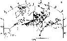
Distribution map of Calanus helgolandicus by geographical zones
|
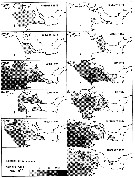
| | | | | | | | | 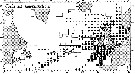 issued from : R. Williams in Bull. mar. Ecol., 1972, 8. [p.55, Fig.1]. issued from : R. Williams in Bull. mar. Ecol., 1972, 8. [p.55, Fig.1].
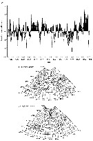
Ditribution of stages V and VI in the North Atlantic from the Continuous Plankton Recorder.
The chart show the average abundance and distrubution derived from more than 43.000 samples taken a depth of 10 m during 1958 to 1968. The samples were assigned to rectangles of 1° lat. by 2° long. The boundary of the sampled area (defined as those rectangles sampled in more than 5 months) is shown by the straight lines in the chart; within this area the average abundance in each rectangle is shown by circular symbols; the presence of the species in the occasional samples outside this area is indicated by plus signs. The absence (in the sampled area) indicates that the species was not found in CPR.
large and small filled in circles and open circles, respectively, are used to indicate the following categories of abundance (average numbers per sample of 3.3 m3: >0.60 : 0.60-0.10 : <0.10 |
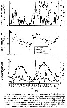
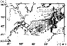 issued from : R. Williams in Mar. Biol., 1985, 86. [p.147, Fig.3]. issued from : R. Williams in Mar. Biol., 1985, 86. [p.147, Fig.3].
Calanus helgolandicus. Annual mean distribution and abundance from sampling at 10 m depth by the Continuous Plankton Recorder. Data for all months sampled from 1960 to 1981. The boudary of the sampled area is shown by straight lines. Position of the 14°C isotherm in August is shown. |
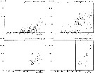
 issued from : R. Williams in Mar. Biol., 1985, 86. [p.148, Fig.6]. issued from : R. Williams in Mar. Biol., 1985, 86. [p.148, Fig.6].
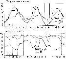
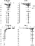
Calanus finmarchicus (a) and C. helgolandicus (b) from Celtic Sea (53°30'N, 07°00'W). Vertical distribution of Copepodite V and VI. Numbers in each night (black) and day (white) hauls are plotted in 5 m depth intervals as percentagges of total numbers (n) present in the haul.
Temperature and Salinity profiles are shown for the day hauls. GMT: Greenwhich Mean Time.
Nota: The two congeneric copepods are morphologically very similar and show little phenotypic divergence. No hybrids are produced between the species which demonstrates that their isolating mechanisms are fully evolved. The only reason that C. finmarchicus, a northern species, is able to persist in the Celtic Sea, which has a sea-surface temperature of ca. 18° C, is because the sea becomes seasonally thermally stratified and a winter sea-temperature is retained below the thermocline. |
 issued from : U. Brenning in Wiss. Z. Wilhelm-Pieck-Univ. Rostock - 30. Jahrgang 1981. Mat.-nat. wiss. Reihe, 4/5. [p.3, Figs.4, 5]. issued from : U. Brenning in Wiss. Z. Wilhelm-Pieck-Univ. Rostock - 30. Jahrgang 1981. Mat.-nat. wiss. Reihe, 4/5. [p.3, Figs.4, 5].
Spatial distribution and T-S Diagram for Calanus helgolandicus from 8° S - 26° N; 16°-20° W, for different expeditions (V1: Dec. 1972-Jan. 1973; IV: Jun.-Jul. 1972; V: Feb.-Mar. 1973; VI: May 1974).
SO: Southern Surface Water (S °/oo: 34,50; T°C: 29,0); ND: Northern Water of the Surface Layer (S °/oo: 37,5; T°C: 21,0); SD: Southern Deep Water of the surface layer (S °/oo: 35,33; T°C: 13,4).
Water types basing on the works of Sverdrup & al. (1942), Wolf (1978) and Wolf & Kaiser (1978) distinguishing various quasi-permanent water types in the top 200 m of the water column in the NW Africa upwelling region. The water type SD, which usually forms the upper limit of the SACW (South Atlantic Central water: S °/oo: 34,35-35,33 & T°C: 5,15-13,4), can enter the surface layer as a result of upwelling, so that water types ND, SD and SO can be expected in this layer in upwelling regions. The boundary separating the NACW (North Atlantic Central Water: S °/oo: 35,10-37,35; T°C: 8,0-21,0) and SACW water masses is situated in the region between Bahia de Gorrei and Cap Blanc (Mauritania) throughout the whole year. The distribution of the water types SACW in the surface layer off North West Africa varies with the season and the meridional migration of the wind field. See in Brenning (1985 a, p.6). |
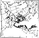 issued from : W.A. Jaschnov in Int. Revue ges. Hydrobiol., 1970, 55 (2). [p.205, Fig.3] issued from : W.A. Jaschnov in Int. Revue ges. Hydrobiol., 1970, 55 (2). [p.205, Fig.3]
Distribution of Calanus helgolandicus from literary sources and unpublished data.
Solid lines indicate the boundaries of Mediterranean water of definite salinity 36.0- 35.5 and 35.0 p.1000 (Defant, 1955. Arrows denote some of the currents. Dark circles indicate occurrence in reproduction areas, semi-dark circles in immigrated areas and white circles in expatriation areas (usual single findings). |
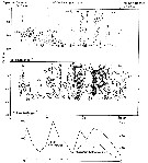
 issued from : R. Gaudy in Tethys, 1972, 4 (1). [p.237, Fig.36]. issued from : R. Gaudy in Tethys, 1972, 4 (1). [p.237, Fig.36].
Schematic quantitative abundance of Calanus helgolandicus in the Gulf of Marseille (Mediterranean Sea) established from samples during the period between February 1961 to June 1967.
Gaudy (p.220) points to 3 generations per year in the neritic province from the winter to the spring, plus probably 2 generations off shore and deeper water (funding the mean development time determined graphically from nauplii to adults for the first three generations between 30 to 75 days); considering a mean development time of 45 days, interval separating two generations should be estimated 75 days; in consequence of the period August-December permitted a development of two genarations. |
 issued from : S. Eriksson in ZOON, 1973, 1. [p.46, Fig.9]. issued from : S. Eriksson in ZOON, 1973, 1. [p.46, Fig.9].
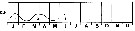
Size distribution of adult females of Calanus helgolandicus (offshore station H6:11°30'N, 57°40'.5, The Kattegatt) during 1969-70 in the main series. |
 issued from : S. Eriksson in Mar. Biol., 1974, 26. [p.320, Figs. 2-3] issued from : S. Eriksson in Mar. Biol., 1974, 26. [p.320, Figs. 2-3]
Salinity and temperature curves for main series at offshore station H6 (11°30' N, 57°40'.5 E, The Kattegatt) from March 1968 to November 1970. |
 Issued from : E.D.S. Corner & S.C.M. OHara in The Biological chemistry of Marine Copepod, 1986. [p.305, Fig.6.10]. Issued from : E.D.S. Corner & S.C.M. OHara in The Biological chemistry of Marine Copepod, 1986. [p.305, Fig.6.10].
Diagrammatic representation of gross differences in the gut epithelium of (A) non feeding and (B) feeding Calanus helgolandicus. From Nott & al., 1985 ; copyright Springer-Verlag, 1985.
Nota : For the authors, gross cyrtological differences between cells of the digestive epithelium of feeding and non-feeding C. helgolandicus showed a spent vacuolated cell disintegrating into the mid-gut lumen, its membranous contents clearly visible (B).
One interesting characteristic of the cells lining the gut, and one especially relevant to the presence of the animals own lipids in its faecal pellets, is the tendency of these epithelial cells to rupture during the digestive process and release cellular material into the lumen of the gut, where it would mix with undigested food. Such a mechanism may well account for lipids characteristic of the animal, sepecially fatty acids and cholesterol, becoming incorporated in faecal pellets, so providing the animals signature on their lipid content. The re-absorption of cell contents of disrupted digestive epithelium by the R cells of the distal region (zone III) is likely to be an inefficient process.
In conclusion, the pelagic food webs constitute the link between the production and deposition of biolipids in the ocean. Copepods in particular have been shown to occupy a key position , as their faecal pellets contribute to sedimentary particulate material, especially in oceanic areas. Faecal pellets transport living material to the deep sea (see in Urrère & Knauer, 1981 ; Silver & Alldredge, 1981 ; Silver & Bruland, 1981 ; Fowler & Fisher, 1983). Such a mechanism has also been found to apply to the distribution of certain bacteria in the water column, these bacteria developing in the guts of animals and then being released in faecal material. Gowing & Silver (1983) regard these internal bacteria as facultative anaerobes, resistant to digestion and originating deep inside the pellets during their formation. Earlier, Silver & Alldredge (1981) observed both heterotrophic and autotrophic bacteria, including cyanobacteria, in faecal pellets and their fragments entrapped in fast-sinking marine snow. |
 Issued from : C.J. Corkett in J. exp. mar. Biol. Ecol., 1972, 10. [p.172, Table I]. Issued from : C.J. Corkett in J. exp. mar. Biol. Ecol., 1972, 10. [p.172, Table I].
Development time to hatching of eggs of Calanus helgolandicus.
Animals collceted off Plymouth (English Channel) on 24th May 1971.
Nota: The rate of development of eggs shows that the development time increases with decreasing temperature.
Corkett points to the larger eggs of C. hyperboreus (190 µ, after McLaren & al., 1969) and C. glacialis (178.6 ±2.5 µ, after McLaren, 1966) take longer to develop than the smaller eggs of C.finmarchicus (145 µ, after Marshall & Orr, 1953) and C. helgolandicus (163.9 ±0.866 µ at Plymouth).
A possible explanation for the linear relationship is that that development rate is determined by the surface : volume ratio which decreases with increasing diameter.
One could think that the metabolic exchange between the egg and its external environment is relatively slower for the larger eggs with their relatively smaller surface. Alternatively, one might assume that the development rate is determined by metabolic processes related to the size of the internal surfaces which in turn is proportional to the external surface. |
 issued from : N.R. Collins & R. Williams in Mar. Biol., 1981, 64. [p.282, Fig.11]; issued from : N.R. Collins & R. Williams in Mar. Biol., 1981, 64. [p.282, Fig.11];
Calanus helgolandicus. Monthly distribution and abundance in Bristol Channel and Severn Estuary from November 1973 to February 1975, together with 33 p.1000 S isohaline. |
 issued from : N.R. Collins & R. Williams in Mar. Biol., 1981, 64. [p.283, Fig.12]; issued from : N.R. Collins & R. Williams in Mar. Biol., 1981, 64. [p.283, Fig.12];
Calanus helgolandicus. Numerical abundance plotted against salinity for the four seasons in Bristol Channel and Severn Estuary from November 1973 to February 1975; 33 p.1000 S value is indicated.
Nota: This stenohaline species was found mostly in the southwestern area of the survey and was carried into the Channel by incursion of high salinity water from the Celtic Sea. Over most of the sampling period the approximate limit of penetration of the species into the Channel was represented by the position of the 33 p.1000 S isohaline, although in the spring it penetrated furyher up the Channel, close to the 30 p.1000 S isohaline. |
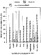 Issued from : M. Laabir, S.A. Poulet, A. Ianora, A. Miralto & A. Cueff in Mar. Ecol. Prog. Ser., 1995, 129. [p.99, Fig.3]. Issued from : M. Laabir, S.A. Poulet, A. Ianora, A. Miralto & A. Cueff in Mar. Ecol. Prog. Ser., 1995, 129. [p.99, Fig.3].
Calanus helgolandicus (from Roscoff, France). Histograms of the relative proportions of diatoms, non-diatoms plus debris and bacteria estimated in the faecal pellets of wild females.
Each bar corresponds to the mean of at least 3 selected samples per month during 1993. |
 Issued from : G.A. Robinson, J. Aiken & H.G. Hunt in J. mar. biol. Ass. U.K., 1986, 66. [p.213, Fig.10]. Issued from : G.A. Robinson, J. Aiken & H.G. Hunt in J. mar. biol. Ass. U.K., 1986, 66. [p.213, Fig.10].
Temperature and chlorophyll sections and plankton from a tow by Undulating Oceanographic Recorder (Aiken, 1981) on 23 August 1979 along the transect route Plymouth -Roscoff (west English Channel).
Scales for total copepods (x 10 power 4) on left and for C. helgolandicus on the right. |
 Issued from : A. Fleminger & K. Hulsemann in Mar. Biol., 1977, 40. [p.245, Table 4]. Issued from : A. Fleminger & K. Hulsemann in Mar. Biol., 1977, 40. [p.245, Table 4].
Length of prosome (mm) and number of teeth on coxopodite of P5 in adult females selected at random from samples used to determine urosome pore signature. |
 Issued from : A. Fleminger & K. Hulsemann in Mar. Biol., 1977, 40. [p.241, Fig.5 a]. Issued from : A. Fleminger & K. Hulsemann in Mar. Biol., 1977, 40. [p.241, Fig.5 a].
Distribution of Calanus helgolandicus sensu stricto in North Atlantic and adjacent seas based on published litterature (squares: Edinburg Oceanographic Laboratory, 1973; open triangles: Jaschnov, 1970; present records: circles). Stippled areas approximate inhabited region beyond or at perimeter of North Atlantic Ocean. |
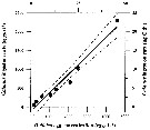 Issued from : A. Lopez-Urrutia, R.P. Harris & T. Smith in Limnol. Oceanogr., 2004, 49 (1). [p.304, Fig.1]. Issued from : A. Lopez-Urrutia, R.P. Harris & T. Smith in Limnol. Oceanogr., 2004, 49 (1). [p.304, Fig.1].
Calanus helgolandicus feeding on Oikopleura dioica eggs, from off Plymouth (English Channel.
Lines represent the least square regression (slope = 0.490 ± 0.039; intercepts = - 1.16 ± 0.82 (µg Cby day) and 116 ± 82 (eggs by day); ± SE; r2 = 0.96; n = 8; P < 0.001 and 95% confidence limits for the parameter estimates (dashed lines). |
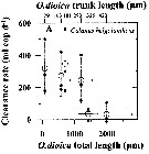 Issued from : A. Lopez-Urrutia, R.P. Harris & T. Smith in Limnol. Oceanogr., 2004, 49 (1). [p.305, Fig.3]. Issued from : A. Lopez-Urrutia, R.P. Harris & T. Smith in Limnol. Oceanogr., 2004, 49 (1). [p.305, Fig.3].
Clearance rate of (A) Calanus helgolandicus from off Plymouth (English Channel), in relation to the size of Oikopleura dioica (Appendicularians).
The first x-axis data points represent the diameter of O. dioica eggs. Solid symbols represent the measured clearance rates and open symbols represent their mean. Vertical and horizontal error bars are the standard deviation of clearance rates and O. dioica size, respectively.
O. dioica cultures were maintened and experiments conducted in a constant temperature room at 15°C with a simulated 12:12 day: night cycle. Cohorts of cultured O. dioica , maintened according to Fenaux and Gorsky, 1985, were used to obtain eggs and juvenile appendicularians. |
 Issued from : M. Cole, P. Lindeque, E. Fileman, C. Halsband, R. Goodhead, J. Moger & T.S. Galloway in Environ. Sci. Technol., 2013, 47. [p.66,49, Fig.1, i]. Issued from : M. Cole, P. Lindeque, E. Fileman, C. Halsband, R. Goodhead, J. Moger & T.S. Galloway in Environ. Sci. Technol., 2013, 47. [p.66,49, Fig.1, i].
Calanus helgolandicus containing 20.6 µm polystyrene beads (dorsal view), visualized using fluorescence microscopy;
Scale bar (gray line): 100 µm. |
 Issued from : E.F. Møller, M. Maar, S.H. Jonasdottir, T.G. Nielsen & K. Tönnesson in Limnol. Oceanogr., 2012, 57 (1). [p.214, Fig.1]. Issued from : E.F. Møller, M. Maar, S.H. Jonasdottir, T.G. Nielsen & K. Tönnesson in Limnol. Oceanogr., 2012, 57 (1). [p.214, Fig.1].
Experimental data and the fitted function on clearance rate (mL./ Copepode/day) of (a) Calanus helgolandicus (R2 = 0.57, p <0.001) and (b) Calanus finmarchicus (R2 = 0.45, p <0.001) as a function of temperature. Error bars are SD. (c) Clearance rate for both species normalized to fraction of its maximum.
For parameter values see Table 1.
Nota: The ingestion response to temperature was determined in the laboratory where the copepods were fed the diatom Thalassiosira weissflogii.
C. finmarchicus from Gullmar fjord (58°19.2'N, 11°32.8'E) on 06 April 2009; C. helgolandicus from off Plymouth (U.K.) in June 2009.
C. finmarchicus develops faster than C. helgolandicus below 11°C and slower above. The different relative development rates of the species are related to different temperature responses in ingestion rates.
A temperature increase of 1°C to 2°C may have consequences for the relative contribution of the two species to the copepod community, and both seasonal and spatial displacements of the Calanus populations can be expected under climate change. |
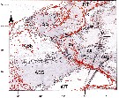 Issued from : N. McGinty, A.M. Power & M.P. Johnson in J. Exp. Mar. Biol. Ecol., 2011, 400. [p.125, Fig. 2]. Issued from : N. McGinty, A.M. Power & M.P. Johnson in J. Exp. Mar. Biol. Ecol., 2011, 400. [p.125, Fig. 2].
Locations of the ten clusters defined as ecosystem regions by K-means partitioning of satellite-derived Chl-a data. The locations of CPR samples throughout the study area are marked by black dots. Red contours indicate the underlying bathymetry at 200, 400, 800, 1600 and 3200 m intervals. Abbreviations and attributes that relate to each region are described in Table I.
Nota: Calanus finmarchicus is a sub-polar species whose presence in an area indicates a cold water influence while its congener, Calanus helgolandicus is seen as a more temperate oceanic species. These two species are used to test the inter-regional variation in the northern Atlantic. Only the adult stages (CV-CVI) are differentiated to species level.
Changes in phenology are implied when there is a significant month by time interaction. The centre-of-gravity date for seasonal zooplankton abundance was used as a measure of the timing of the seasonal peak, also known as the central tendency (T) is sensitive to monthly changes in abundance and can be viewed as a measure of the phenological change in the species annual cycle over time. T is estimated in decimal month units. See Beare & McKensie; 1999; Edwards & Richardson, 2004; Richardson & al., 2006.
Changes in sea surface temperature (SST) represent a strong environmental proxy for measuring climate related changes as this variable affects zooplankton at both the macro-ecological and the physiological level (SST data came from the HadISST1 dataset, provided by the Hadley Centre for Climate Prediction and Research Meterological Office, London, UK (Rayner & al., 2003).
Following the Chl-a based clustering, the long term SST pattern was compared among regions. The long term trend in SST was estimated from the slope of a linear regression of standardized SST against year. Variations in the link between SST and the dominant modes for the overall study area Atlantic Multidecadal Oscillation (AMO), the East Atlantic Pattern (EAP), and the North Atlantic Oscillation (NAO) index; (Cannaby & Husrevoglu, 2009) were examined using best fit regressions.
All the regions showed a warming trend over the time period considered:
- Warming was greatest in the Celtic Sea (CS) and Celtic mixed (CM) regions of shelf, at the Shelf Edge and in the more southern and central oceanic regions (WT, ABS and ABN; see Table 1).
- The influence of modes of variability affecting SST varied among regions. The AMO, itself a temperature signal, was present in all areas. The influence of climate indices varied, with the NAO a positive influence on SST in southern shelf and ocean regions and Irish Sea, but absent or with a negative association in central and northern off-shelf regions and Main Shelf (MS).
- The East Atlantic Pattern (EAP) was only selected as part of the best fit model in the Rockall Trough (RT) region.
The central tendency (T) for spatially averaged Chl-a in each region was calculated using values from March-October for each year. Off-Shelf there was a general northward progression in the timing of the seasonal peak.
- The earliest peak occurred in the Warm Temperate region (mean T of 5.76) with a gradual progression towards later seasonal peaks in the more northward regions. There was a difference of nearly a month between the most southern region, WT, and the two northern regions RT and RB, which had mean T of 6.61 and 6.64 months respectively.. On shelf there was less of a difference between the earliest and latest seasonal peak. The earliest T (SE) was 6.21 months while the latest (6.49 months) occurred in the Celtic Mixed (CM) region |
 Issued from : N. McGinty, A.M. Power & M.P. Johnson in J. Exp. Mar. Biol. Ecol., 2011, 400. [p.124, Table 1]. Issued from : N. McGinty, A.M. Power & M.P. Johnson in J. Exp. Mar. Biol. Ecol., 2011, 400. [p.124, Table 1].
Ecosystem regions of the northen Atlantic studied by CPR. Data for all months between 1998 and 2008.
Nota: The measure of phenology, T, varied within and between regions over time.
For C. helgolandicus, the mean T was 6.4 months with an average range within of 1.2 months C. finmarchicus generally had the earliest central tendancy (5.7 months), and their average range was slightly larger (mean range 1.6 months).
In the majority of cases, increases in regional SST anomaly were negatively associated with the timing of the seasonal abundance peak (Fig.4, time series shown in Fig.5). This implies an earlier zooplankton ''bloom'' in warmer years. There were a few exceptions where this negative relationship with SST failed to hold. For C. helgolandicus, the region WT showed a relatively small correlation between ce,ntral tendaency and SST. For C. finmarchicus, the IS region had a weak positive correlation.
The annual average abundance of C. helgolandicus tended to be higher in warm years, with a positive correlation between abundance and SST in all areas except IS and SE. The strongest positive associations with temperature were in the northern regions of RT and MS. The pattern of mostly positive associations between annual copepod abundance and annual SST anomaly was reversed in the majority of cases in C. finmarchicus. |
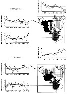
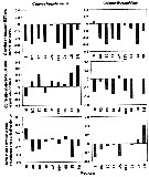 Issued from : N. McGinty, A.M. Power & M.P. Johnson in J. Exp. Mar. Biol. Ecol., 2011, 400. [p.126, Fig. 4]. Issued from : N. McGinty, A.M. Power & M.P. Johnson in J. Exp. Mar. Biol. Ecol., 2011, 400. [p.126, Fig. 4].
Correlations betweej the timing of seasonal abundance peak (T) and standardized SST anomaly (first row), annual average abundance and standardized SST anomaly (second row) and annual average abundance and timing (last row) for each taxon. Gaps in the charts for the correlation between T and SST are where model fitting did not indicate an interaction between month and year. |
 Issued from : N. McGinty, A.M. Power & M.P. Johnson in J. Exp. Mar. Biol. Ecol., 2011, 400. [p.127, Fig. 5]. Issued from : N. McGinty, A.M. Power & M.P. Johnson in J. Exp. Mar. Biol. Ecol., 2011, 400. [p.127, Fig. 5].
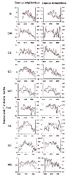
The central tendency (T) in decimal months, for Calanus helgolandicus and C. finmarchicus (black line) and local SST (red line) for each of the nine ecosystem regions.
Where zooplankton abundances varied between bimodal and unimodal peaks, only the unimodal pattern is shown. SST anomalies are inverted on the y axis. Abbreviations of each ecosystem regions are given in full in p.124, Table I. |
 Issued from : N. McGinty, A.M. Power & M.P. Johnson in J. Exp. Mar. Biol. Ecol., 2011, 400. [p.128, Fig. 6]. Issued from : N. McGinty, A.M. Power & M.P. Johnson in J. Exp. Mar. Biol. Ecol., 2011, 400. [p.128, Fig. 6].
Mean accepted numbers (3 per m3) for Calanus helgolandicus in the nine ecosystem regions (three year running mean).
Note the scales differ. |
 Issued from : C. Wexels Riser, S. Jansen, U. Bathmann & P. wassmann in Mar. Ecol. Prog. Ser., 2003, 256. [p.303, Fig.2] Issued from : C. Wexels Riser, S. Jansen, U. Bathmann & P. wassmann in Mar. Ecol. Prog. Ser., 2003, 256. [p.303, Fig.2]
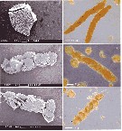
Scanningt electrom micrographs (SEM) of (a) Dinophysis norvegica, (b, c) Calanus helgolandicus faecal pellet containing D. norvegica; (d-f) light micrographs of C. helglandicus pellets containing D. norvegica.
Nota: Production rate of faecal pellets by individual and by day = 23.6 ± 1.6; faecal pellet volume produced (mm3 by ind. by day) = 0.026 ± 0.010; faecal pellet carbon produced (µg C by ind. by day) = 1.82 ± 0.75.
Faecal pellet length (µm) = 374 ±5.0; faecal pellet diameter (µm) = 65.9 ±0.4; faecal pellet volume (x 10000 µm3). |
 Issued from : H. Bi, K.A. Rose & M.C. Benfield in Mar. Ecol. Prog. Ser., 2011, 427. [p.157, Table 5]. Issued from : H. Bi, K.A. Rose & M.C. Benfield in Mar. Ecol. Prog. Ser., 2011, 427. [p.157, Table 5].
Instantaneous mortality rates (individuals per day) from litterature. |
 Issued from S. Razouls in XXIII rd Congress of Athens, 3-11 November 1972. [p.2]. Oxygen consumed by individual (adult) in the Banyuls Bay. Issued from S. Razouls in XXIII rd Congress of Athens, 3-11 November 1972. [p.2]. Oxygen consumed by individual (adult) in the Banyuls Bay.
(1) Hydrological season in the stability period: Eté = Summer: 18-20 °C; Hiver = Winter: 13-10°C.
Espèces = species; Saison = Season; Lg céph.= cephalothoracic length; an = individual. |
 Issued from : A.G. Hirst, D. Bonnet & R.P. Harris in Mar. Ecl. Prog. Ser., 2007, 340. [p.195, Fig.4]. Issued from : A.G. Hirst, D. Bonnet & R.P. Harris in Mar. Ecl. Prog. Ser., 2007, 340. [p.195, Fig.4].
Calanus helgolandicus egg production and surface water temperature and surface chlorophyll a concentration in the English Channel at Station L4 from March 2002 to March 2004 |
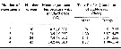
 Issued from : H. Saito & A. Tsuda in Deep-Sea Res. I, 47. [p.2146, Table I]. Issued from : H. Saito & A. Tsuda in Deep-Sea Res. I, 47. [p.2146, Table I].
Egg diameter, carbon and nitrogen content, and prosome length (PL) of females of Calanus helgolandicus after Uye (pers. comm.): c, Pond & al., 1996: f, McLaren & al., 1988: e.
Nota: Compare with N. cristatus, N. tonsus and N. flemingeri and others species in genus Calanus. |
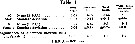
 Issued from : C.J. Corkett, I.A. McLaren & J.-M. Sevigny in Syllogeus, 1986, 58. [p.545, Table I]. Issued from : C.J. Corkett, I.A. McLaren & J.-M. Sevigny in Syllogeus, 1986, 58. [p.545, Table I].
Relative times to reach various stages of C. helgolandicus, assuming equiproportional development.
All times expressed relative to time between hatching and molting to CI.
2 : From Thompson (1982, Tables 2, 6; mean proportions for all temperatures except 4.5° and 13.9°C, for which data are incompleted.
Nota: Compare with Calanus hyperboreus, C. finmarchicus , C. glacialis and C. pacificus. |
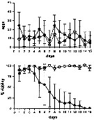 Issued from : A. Ianora & A. Miralto in Ecotoxicology, 2010, 19. [p.503, Fig.3]. Issued from : A. Ianora & A. Miralto in Ecotoxicology, 2010, 19. [p.503, Fig.3].
Unpublished results showing daily mean egg production rates (±SD) and percent egg viability for Calanus helgolandicus females (n= 15 replicates) maintained for 15 days on monoalgal diatom diets of the non-PUA (polyunsatured aldehydes and others oxylipins) producing pennate diatom Pseudo-nitzchia delicatissima (black circles) and control diets od the dinoflagellate Prorocentrum minimum (white circles).
There were no statistical differences between the two diets in terms of egg productionrates (t28 = 1.77; P > 0.05) but highly significant differences were found in terms of egg hatching success (t28 = 6.25; P < 0.0001).
Experimental protocols to measure egg production and egg viability are the same as in Turner & al., 2001;
Food concentrations tested were 10 power 4 cells per ml. |
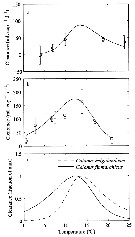
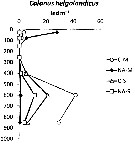 Issued from : I. Siokou, S. Zervoudaki & E. D. Christou in J. Plankton Res., 20013, 35 (6). [p.1319, Fig.5]. Issued from : I. Siokou, S. Zervoudaki & E. D. Christou in J. Plankton Res., 20013, 35 (6). [p.1319, Fig.5].
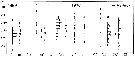
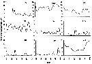
Vertical distribution of Calanus helgolandicus abundance (ind.m3 in the Aegean Sea, 1997.
NA-M: mean over stations N Aegean Sea in march; NA-S: mean over stations in September; C-M: station in March: C-S: station in September.
Nota: C. helgolandicus, large copepod, had specific vertical patterns with Subeucalanus monachus. The former was abundant in the 0-100 m layer in the northern Aegean Sea (87 ind.m3 and 3.5% of copepods) and it declined down to 300 m. It reappeared <300 m (41.6 ind.m3 in the 500-700 m layer, representing 67% copepods). In contrast, it was very rare in the surface and deepest layers in the south.
See profiles temperature and salinity. |
 Issued from : I. Siokou, S. Zervoudaki & E. D. Christou in J. Plankton Res., 20013, 35 (6). [p.1315, Fig.2]. Issued from : I. Siokou, S. Zervoudaki & E. D. Christou in J. Plankton Res., 20013, 35 (6). [p.1315, Fig.2].
Mean temperature and salinity profiles (Standard deviations are shown by horizontal lines) in the Aegean Sea in March (upper) and September (lower), 1997.
NA: north Aegean Sea; SA: south Aegean Sea. |
 Issued from : P. Helaouët & G. Beaugrand in Mar. Ecol. Prog. Ser., 2007, 345. [p.152, Fig.3, b]. Issued from : P. Helaouët & G. Beaugrand in Mar. Ecol. Prog. Ser., 2007, 345. [p.152, Fig.3, b].
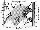
Spatial distribution in North Atlantic Ocean Calanus helgolandicus. No interpolation made.
Data on the abundance of copepods provided by the Continuous Plankton Recorder (CPR) survey, a large-scale plankton monitoring programme initiated by Sir Alister Hardy in 1931. CPR towed at a depth of 7 m (see in Reid & al., 2003) and investigated the area from Longitude 99.5°W to 19.5°E and Latitude 29.5° to 69.5°N.
See the same authors, text and figures in Calanus finmarchicus.
The target of the study of the two species C. helgolandicus and C. finmarchicus is how the Global climate change modifies the spatial distribution and projections of future changes should be based on information on the ecological niche sensu Hutchinson (1957), i.e. the field of tolerance of a species to the principal factors of its environment.
Eleven parameters were chosen including bathymetry, temperature, salinity, nutrients, mixed-laye(r depth and an index of turbulence compiled from wind data and chlorophyll a concentrations (used herein as an index of available food).
The most important parameters that influenced abundance and spatial distribution were temperature and its correlates such as oxygen and nutrients.
Bathymetry and other water-column-related parameters also played an role.
The ecological niche of C. finmarchicus was larger than that of C. helgolandicus and both niches were significantly separated. C. finmarchicus appears to be a good indicator of the Atlantic Polar Biome (mainly the Atlantic Subarctic and Arctic provinces) while C. helgolandicus is an indicator of more temperate waters (Atlantic Westerly Winds Biome) in regions characterized by more pronounced spatial changes in bathymetry. |
 Issued from : P. Helaouët & G. Beaugrand in Mar. Ecol. Prog. Ser., 2007, 345. [p.163, Fig.16]. Issued from : P. Helaouët & G. Beaugrand in Mar. Ecol. Prog. Ser., 2007, 345. [p.163, Fig.16].
Infuence of different abiotic variables on Calanus finmarchicus and Calanus helgolandicus.
Nota: A remarkable feature of the authors' study is that the environmental optimum of Calanus species varies seasonally for all abiotic parameters. Theses seasonal fluctuations might be influenced by the spatial variability in the seasonallity of both species (Planque & al., 1997).
For C. finmarchicus, seasonal fluctuations could be related to large-scale differences in the timing of ontogenetic vertical migration. Another hypothesis is that they could be related to the differential sensivity of the mean developmental stages of Calanus population to temperature that has been observed in some experiments (Harris & al., 2000)
The use of this 'ecological niche approach' has allowed an explanation of the shift in Calanus dominance to be outlined. Reid & al. (2003b) showed a substantial and sustained reduction in the percentage contribution of C. finmarchicusCalanus in the North Sea. While in 1962, C. finmarchicus comprised 80% of Calanus spp. in the North Sea, C. helgolandicus comprised 80% of Calanus identified by the Continuous Plankton Recorder (CPR) survey in 2000.
Calanus dominance in the North Sea is highly sensitive to temperature, especially in spring and summer. The authors have demonstrated that the shift in dominance could have been triggered solely by temperature changes in the North Sea. Sea surface tepmperature (SST) changes are likely to be related to changes in ai(r temperature (Beaugrand, 2004b) over the region and changes in advection recently discussed in Reid & al. (2003b). Reid & al. (2003b) reported that when the North Atlantic Oscillation (NAO) was positive, the strength of the European shelf-edge current, which flows northwards, increased and that oceanic inflow into the northern part of the North Sea was strengthened.
During the cold regime in the North Sea prior to 1980, this region was the boundary between a subarctic biome and a more temperate biome (Longhurst, 1998).
As C. finmarchicus is indicative of the Atlantic Arctic buiome, the change in the proportion of Calanus in the North Sea may indicate ythat the subarctic biome has moved northwards.
A northward movement of plankton has been detected using calanoid copepods in the northeastern part of the North Atlantic (Beaugrand & al., 2002) and a similar shift has been found for fish (Perry & al., 2005).
The authors showed the usefulness of Hutchinson's ecological niche concept. However, it is important to note that after the authors' study, they assessed the realised, not the fundamental, 'niche' of Calanus spp. Hutchinson (1957) made this distinction and stated that the realised 'niche' should always be smaller than the fundamental 'niche' as species interactions eliminate individuals from favourable biotopes. However, Pulliam (2000) recently showed that when dispersal is high, the realised 'niche' can be larger than the fundamental 'niche'. |
 Issued from : C.B. Miller in Biological Oceanography, Blackwell Publishing, 2004/2005. [p.357, Fig.16.11]. After Planque & Ibanez, 1997. Issued from : C.B. Miller in Biological Oceanography, Blackwell Publishing, 2004/2005. [p.357, Fig.16.11]. After Planque & Ibanez, 1997.
Variation of Calanus helgolandicus and C. finmarchicus abundance in the North Sea, Norwegian Bight (west of southern Norway and Faeroes-Iceland sector 1958-1996. |
 Issued from : C.B. Miller in Biological Oceanography, Blackwell Publishing, 2004/2005. [p.358-59, Fig.16.12 a, b]. Issued from : C.B. Miller in Biological Oceanography, Blackwell Publishing, 2004/2005. [p.358-59, Fig.16.12 a, b].
(a) Time series of the North Atlantic Oscillation (NAO) index estimates for 1860 to 2000.
NAO is the atmospheric presure difference between Iceland and Portugal, plotted here as anomalies (From NOAA)
General effects of low NAO (b) and high NAO (c) on ocean current patterns in the North Atlantic (After Mann & Lazier, 1991).
See clearly explanations in the author (p.355-56). |
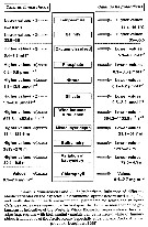
 Issued from : S. Ban, C. Burns, J. Castel, Y. Chaudron & al. in Mar. Ecol. Prog. Ser., 1997, 157. [p.289, Table 1]. Issued from : S. Ban, C. Burns, J. Castel, Y. Chaudron & al. in Mar. Ecol. Prog. Ser., 1997, 157. [p.289, Table 1].
Synopsis of feeding/reproduction experiments. A total of 17 diatom and 16 copepod species, representative of a variety of worldwide temperate and subarctic environments (E: estuarine, C: coastal ocean), were screened.
Data for fecundity and hatching success are average values measured at the start and end of the inciubations in a minimum of 3 replicate batches, showing the variation in time of the effects of diatoms on copepod reproduction.
Level of significance of the diatom effect between treatments and controls (e.g. non-diatom diets) in categories I to III was p < 0.01. No.. rank (for comparison with Table 2, p.290).
For the signification of the categories I to IV (fecundity vs. Hatching success vs. Duration of experiment days-1): See Calanus finmarchicus.
List of the 12 marine or estuarine species studied (fresh water excluded. CR): Acartia clausi, A. grani, A. steueri, A. tonsa, Calanus finmarchicus, C. helgolandicus, C. pacificus, Centropages hamatus, C. typicus, Eurytemora affinis, Temora longicornis, T. stylifera. |
 Issued from : S. Ban, C. Burns, J. Castel, Y. Chaudron & al. in Mar. Ecol. Prog. Ser., 1997, 157. [p.290, Table 2]. Issued from : S. Ban, C. Burns, J. Castel, Y. Chaudron & al. in Mar. Ecol. Prog. Ser., 1997, 157. [p.290, Table 2].
Combinations of copepod and non-diatom diets in controls in concentrations ranging from 104 to 105 cells ml-1. Data for fecundity and hatching success are average values measured at the start and end of incubation in a minimum of 3 replicate batches.
No9: In Category I; Nos 21 and 22: In Category II; Nos 32 and 33: In Category III. |
| | | | Loc: | | | Congo, Morocco-Mauritania, Moroccan coast,Canary Is., off Madeira, Portugal, off W Cape Finisterre, Chesapeake Bay, New-York Bight, off Woods Hole, off Newfoundland, Sargasso Sea, Station "S" (32°10'N, 64°30'W), off SW Ireland, Galway Bay, Lough Hyne, Aran Islands, Ireland, Celtic Sea, Bristol Channel, Rnglish Channel, NE Scotland, Norway, North Sea, Fladen Ground area, Gullmarfjord, Kattegatt, Pas de Calais, English Channel, Plymouth, Roscoff, Bay of Biscay, Arcachon Bay, Gironde estuary, Glenans Islands, Arcachon Bay, Portugal, Mondego estuary, Ria de Aveiro, off Coruña, Vigo, Santander, off Gijon, Cap Ghir, Ibero-moroccan Bay, Morocco, off W Tangier, Medit. (Alboran Sea, Habibas Is, Sidi Fredj Coast, Castellon, Baleares, off Barcelona, Banyuls, Marseille, Villefrance-s-Mer, Ligurian Sea, Tyrrhenian Sea, Naples, Milazzo, G. of Annaba, Strait of Messina, Gulf of Taranto, Malta, Adriatic Sea, Mljet Is., Venezia, Po delta, Aegean Sea, Thracian Sea, Egyptiian coast, Lebanon Sea, Bardawill Lagoon, ? Black Sea) | | | | N: | 352 | | | | Lg.: | | | (22) F: 3,2-2,7; M: 2,8-2,5; (45) F: 3,25-2,75; M: 2,8-2,5; (65) F: 3; M: 2,8; (131) F: 3,5-2,7; M: 3,1-2,5; (180) F: 3,16-2,61; M: 2,58; 2,4; (199) F: 3,31-2,36; M: 3,19-2,36; (207) F: 3,09-2,82; M: 2,59-2,47; (327) F: 3,41-2,4; M: 2,98-2,35; (340) F: 2,8; (373) F: 2,6; (449) F: 5,4-2,7; M: 3,2-2,35; (920) F: 2,654-2,746; (927) F: 2,80-2,86 [winter]; 2,51-2,65 [Fall]; (1009) F: 2,75-3,25; (1037) F: 1,9-2,5; (1107) F: 2,5-3,13; M: 2,5-3,04; (1127) F: 2,6-3,3; M: 2,6-3,0; (1137) F: 2,26-2,57; M: 1,98-3,08; {F: 1,90-3,50; M: 2,35-3,20}
It does'nt take into account the female maximal value very high from Pesta (1920) in the Adriatic Sea.
The mean female size is 2.884 mm (n = 34; SD = 0.5716), and the mean male size is 2.681 mm (n = 23; SD = 0.3247). The size ratio (male : female) is 0.93. | | | | Rem.: | Overall Depth Range in Sargasso Sea: 0-2000 m (most numerous between 1000 and 1500 m) (Deevey & Brooks, 1977, Station"S").
This species has sometimes been confused with C. finmarchicus in the literature, the latter doubtful in the Mediterranean Sea.
In the Pacific it has been replaced by C. sinicus or C. australis, in the southern Atlantic and near South Africa by C. agulhensis.
A doubt subsists in considering C. euxinus as a valid species.
After Vucetic (1965) the number of teeth on coxopodite is for the females 24-26 (23-35), and 16-20 for males, and in C. helgolandicus var. ponticus (Yashnov, 1955) (= Calanus euxinus 24-29 (18-37) for females, and 11-21 for males.
For Itoh (1970 a, fig.2, from co-ordonates) the Itoh's index value from mandibular gnathobase = 370; for Schnack: 370, and for Lapernat & Razouls (2002, p.19) the Itoh's index value = 500.2 (number of teeth: 8).
After Corner & al. (1974) this species could survive the winter in the Clyde sea-area by feeding carnivorously on nauplians forms.
After Benedetti & al. (2018, p.1, Fig.2) this species belonging to the functional group 3 corresponding to large filter feeding herbivorous.
The feeding mode after Barton & al. (2013, Table 1) is 'feeding current' (hovering) (See definition in Rem. Centropages typicus).
See in Mazzocchi M.G., 2006 | | | Last update : 28/10/2022 | |
|
|
 Any use of this site for a publication will be mentioned with the following reference : Any use of this site for a publication will be mentioned with the following reference :
Razouls C., Desreumaux N., Kouwenberg J. and de Bovée F., 2005-2026. - Biodiversity of Marine Planktonic Copepods (morphology, geographical distribution and biological data). Sorbonne University, CNRS. Available at http://copepodes.obs-banyuls.fr/en [Accessed March 15, 2026] © copyright 2005-2026 Sorbonne University, CNRS
|
|
|
|


;)
;)
;)
;)
;)
;)
;)
;)
;)
;)
;)
;)
;)
;)
;)
;)
;)
;)
;)
;)
;)
;)
;)
;)
;)
;)

;)
;)
;)
;)
;)
;)
;)
;)
;)
;)
;)
;)
;)
;)
;)
;)
;)
;)
;)
;)
;)
;)
;)
;)
;)
;)
;)
;)
;)
;)