|
|
 |
|
Calanoida ( Order ) |
|
|
|
Calanoidea ( Superfamily ) |
|
|
|
Calanidae ( Family ) |
|
|
|
Calanus ( Genus ) |
|
|
| |
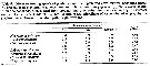
Calanus pacificus Brodsky, 1948 (F,M) | |
| | | | | | | Syn.: | Calanus finmarchicus : Esterly, 1905 (p.125, figs.F,M); 1919 (p.1, 22, light-dark reactions); 1924 (p.83, figs.F,M, Rem.); Sato,1913; Mori,1929; ? Minoda, 1958 (p.253, Table 1); ? M.W. Johnson, 1961 (p.311, Table 2); Motoda, 1966 (p.260);
Calanus finmarchicus pacificus : Kun, 1969 (p.995, fig.F, Rem., chart);
Calanus helgolandicus Mori, 1937 (1964) (p.14, figs.F,M); Nakai, 1955 (p.12, chemical composition); Mullin, 1963 (p.239, Table 2, grazing rate); Ahlstrom & Thrailkill, 1963 (p.57, Table 5, abundance); Furuhashi, 1966 a (p.295, vertical distribution vs mixing Oyashio/Kuroshio region); Mullin & Brooks, 1967 (p.657, life history, fecundity, feeding, growth rate); Mullin C.H., 1968 (p.29, egg laying v.s. hours); Richman & Rogers, 1969 (p.701, feeding); Mullin & Brooks, 1970 (p.748 (p.748, nutrition); Paffenhöfer, 1970 (p.346, cultivation); 1971 a (p.286, feeding); 1976 (p.49, feeding); 1976 a (p.39, feeding);
Calanus finmarchicus s.l. : Morris, 1970 (p.2300).
Calanus helgolandicus (sens. lat.) : Longhurst, 1967 (p.51, fig.3, Table 3, vertical distribution/O2 minimum);
Cf. Calanus pacificus californicus: Brodsky, 1959. | | | | Ref.: | | | Brodsky, 1950 (1967) (part., p.90); Shen & Bai, 1956 (part., p.218, Pl.I: figs.4-6; Brodsky, 1959 a (p.1545, Rem.: var.); 1962 c (p.97); Jaschnov, 1963 (p.1005, biogéo); Brodsky, 1965 (p.2); 1961 (p.15, Rem.); Vinogradov, 1968 (1970) (p.55, 86, 278); Park, 1968 (p.530, figs.F, Rem.); Vaupel-Klein, 1970 (p.3, 5, fig.M, p.41, 42: Tabl. I, II, III, F,M); Minoda, 1971 (p.11); Shih & al., 1971 (p.144); Marshall & Orr, 1972 (p.8); Brodsky, 1972 (1975) (p.9, 66, 81, 119, figs.); Kos, 1976 (Vol. II, figs.F, M); Dawson & Knatz, 1980 (p.5, figs.F,M); Gardner & Szabo, 1982 (p.138, figs.F,M); Brodsky & al., 1983 (p.162, figs.F,M, Rem.); van der Spoel & Heyman, 1983 (p.62, fig.79); Bradford, 1988 (p.74, 76, Rem.); Nishida, 1989 (p.173, fig. 3, table 1, 2, 3 : dorsal hump); Miller & al., 1990 (p.91, figs.: Md); Bucklin & LaJeunesse, 1994 (p.45, molecular genetic variation); Chihara & Murano, 1997 (p.738, Pl.66: F,M); Hill & al., 2001 (p.279, fig.2: phylogeny); Ferrari & Dahms, 2007 (p.34, 35, 36, Rem. N, p.63: copepodites); ); Nuwer & al., 2008 (p.107, Rem.: molecular biology) | 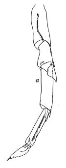 issued from : J.C. von Vaupel Klein in Zool. Verh. Leiden, 1970, 110. [p.5, Fig.1,a]. Male: a, left P5. Nota: P5 of the present male from the weathership \"P\" (50°N, 145°W) is of slightly aberrant type as far as the ratio breadth/length of 1st and 2nd exopodal segments is concerned (1:4.5). Endopod does not reaching distal margin of 1st exopodal segment. In this respect the specimen approaches C. pacificus var. japonicus closest.
|
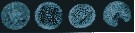
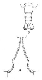 issued from : T. Park in Antarct. Res. Ser. Washington, 1968, 66 (3). [p.531, Pl.1, Figs.3-4]. Female (from Central North Pacific): 3, urosome (dorsal); 4, inner margins of coxae of P5. Nota: the proportional lengths of the prosome and urosome are about 3.28-3.47:1. The genital segment is slightly longer than wide (51:49). The coxa of P5 has 24 to 36 teeth along the inner margin. The distal segment of the endopod of P5 has 5 or 6 setae (as C. glacialis)
|
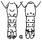 issued from K. Hulsemann in Invert. Taxon., 1994, 8. [p.1477, Fig.28, G]. As Calanus pacificus s.l. Female: G, urosome (left: ventral); right: dorsal). Pore signature schematic by pooled samples (symbols are considerably larger than pores): Filled circle: 100 % presence; open circle: 95-99 % presence; triangle: 50-89 % presence. n = 200.
|
 issued from : G.A. Gardner & I. Szabo in British Columbia Pelagic Marine Copepoda. Canadian Spec. Publ. Fish. Aquat. Sc., 1982, 62. [p.139, Fig.8. 1. 2]. After Woodhouse, 1971. P5Bp1: basipodite 1 of P5.
|
 Issued from : C.B. Miller, D.M. Nelson, C. Weiss & A.H. Soeldner, 1990, 106. [p.97, Fig.6, A, B]. Chewing surfaces of the mandibular gnathobase of copepodite 5 : A, section perpendicular to tooth row, showing a tooth mold early in opal deposition stage (opal is laid down sequentially from distal surface to tooth base; section also shows passage of a 'salivary duct' S adjacent to remains of central cell; B, section showing fusion of a mature fully silicified tooth to underlying chitin ch. Scale bars: 0.006 mm (A); 0.0026 mm (B).
|
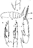 issued from : C.O. Esterly in Univ. Calif. Publs Zool., 1905, 2 (4). [p.125, Fig.1]. As Calanus finmarchicus. Female (from San Diego Region): a, habitus (lateral); e, basipod of P5. Male: b, exopodite of right P5; c, left P5; d, exopodite of P3. St = terminal bristle; Se = outer marginal bristle.
|
 issued from : A. Fleminger in Mar. Biol., 1985, 88. [p.280, Fig.2]. As Calanus pacificus californicus. Male (from off Point Conception, California): A, Left A1 (ventral view), with trithek grouping on segment 4 and quadrithek groupings on segment 5; B, quadrithek female; C, trithek female, with trithek groupings on segments 2b and 5 delincated. Set = seta; aes = aesthetasc. Populations include adult males and two morphological types of adult females, one of which has a first antenna resembling that of the male in the number of aesthetascs. The dimorphism between female types is abrupt, with no intermediate forms, and appears to be genetically founded (no indication seen suggesting that parasitism or disease is responsible for the dimorphism), and the high frequency of quadrithek females rules out an origin from repetitive ordinary mutations. The author postulates that quadrithek females derive from genotypic males in which the gonad develops as an ovary.. The final, phenotypics sex is affected by environmental factors, or possibly by internal factors relating to conditions developed in diapause, which modify the hormonal control of morphogenesis of sexual characters.
|
 issued from : A. Fleminger in Mar. Biol., 1985, 88. [p.281, Fig.3]. As Calanus pacificus californicus. Left A1 (ventral view, segments 16-25. A, Male; B, quadrithek female; C, trithek female.
|
 issued from : A. Fleminger in Mar. Biol., 1985, 88. [p.285, Table 5]. As Calanus pacificus californicus. Aesthetascc variability in A1 of the trithek females. Number of aesthetascs deviating from 1 per antennal segment. In all instances of deviations, 2 aesthetasks were observed; 17 specimens displayed one unilateral deviation, 2 specimens displayed one bilateral deviation. L left; R, right. Nota: The table shows the result for anomalies collected in winter and spring. Very small seviations in aesthetasc number occured in 19 of 200 specimens The morphology of the reproductive system was normal in both trithek and quadrithek females: both morphs showed an advanced state of ovarian development and oviducts filled with eggs. The seminal receptacles always appeared to be filled with sperm, and the antrumn and the cover plate were similar in both morphs. Except for A1, no differences in sexual morphology were noted between trithek and quadrithek females. In samples, quadritheks were more abundant in winter and early spring, their numbers diminishing through midsummer to low in autumn. Quadrithek frequency, prosome length, and population density tended to be high at temperatures below 14°C and vice inversely.
|
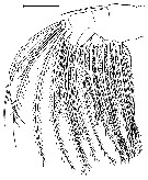 issued from : B.W. Frost in Limnol. Oceanogr., 1977, 22 (3). [p.481, Fig.5]. Female (from puget Sound, Washington): right mx2 (right lateral view). Scale bar: 0.100 mm. Nota: This shows typical orientation of maxillary setae (appendage in formalin-preserved specimen); openings of rather large size, especially in distal part of filter; these would permit escape of rather large single-celled diatoms. observations (measurements of spaces between setae) on fixed specimens incompletely represent the filter structure in the living copepod. The appendage vibrates very rapidly, albeit with much smaller amplitude of motion than the other head appendages. Therefore, during feeding Mx2 are dynamic structures whose total area and size distribution of openings probably vary continually due to temporally variable spacing of the maxillary setae. Also, measurements of maxillary space give no indication of the efficiency with which copepods handle and eat cells that are retained on the Mx2.
|
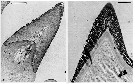
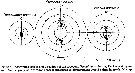
 issued from : K.A. Brodsky in Zool. Zh., 1959, 38, 10. [p.1541, Fig.3, 4-10]. Comparison of coxopodite inner edge of P5 female for Calanus pacificus var. oceanicus (4), C. pacificus var. japonicus (5-9) and C. pacificus var. ? (10) (from Sindao, Yellow Sea). Calanus pacificus var. oceanicus (from N Pacific): Last thoracic segment has small, slightly divergent protuberances. Coxopodite dentate plate of P5 with teeth long, almost parallel sides, closely set; well marked curve in central part of teeth-, in distal part teeth point towards distal part of leg. Number of teeth high: 32-39. Calanus pacificus var. japonicus (from Tartar Straits, off shores of Sakhalin): Forehead in lateral view without protuberance, but is smoothly rounded. Last thoracic segment has short, divergent angles when viewed dorsally. Coxopodite dentate plate of P5 has sharp, closely set teeth without spaces. Central part of teeth-line has strongly marked curve; in some instances the teeth are seen end on (Fig.3-5). The degree of variability of the structure of the dentate plate is shown in Fig.3, 5-8. Number of teeth 22- 29. Population from Amur Bay, Sidimi Bay, Posyet Bay and Melkovodny Bay do not differ from specimens from Tartar Straits as shown in figure 3-9. Calanus pacificus var. ? (from Sindao): Form of body somewhat different from that from Yellow Sea: in dorsal view prominent protuberance is visible forehead, this is noticeable in lateral view. Rear angles of last thoracic segment short and divergent. A1 somewhat shorter than in other populations and do not exceed the length of the body but are equal to it.Coxopodite dentate plate of P5 (Fig.3-10) has sharp, triangular teeth, witout spaces; in central part of teeth-line, to be more precise in the distal third, a curve is noticeable; distal teeth are longer and distally orientated; number of teeth not high 18-20.
|
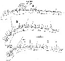
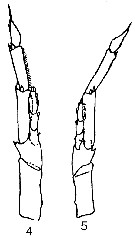 issued from : K.A. Brodsky in Zool. Zh., 1959, 38, 10. [p.1542, Fig.4]. Comparison of left leg of P5 for Calanus pacificus var. oceanicus (4) and C. pacificus var. japonicus (5). Calanus pacificus var. oceanicus (from N Pacific): Segments of exopodite of left P5 are thinner and more elongated than in C. helgolandicus and C. finmarchicus. Relation of breadth to length of 1st and 2nd segments of exopodite of left leg 1 : 3.5. Endopodite almost reaches distal end of 1st segment of exopodite of same leg, and if it is goes beyond, then it is only by a very little (Fig.4-4). Calanus pacificus var. japonicus (from Tartar Straits, off shores of Sakhalin): P5 is of ''thin'' type compared to C. helgolandicus and C. finmarchicus. Relation of breadth to length of 1st and 2nd segments of left exopodite of P5 1 : 4.5. Left endopodite of P5 shorter than 1st segment of exopodite. calanus pacificus var. ? (from Sindao): P5 does not differ from that described for the form from the open part of the Pacific ( C. pacificus var. oceanicus).
|
 Issued from : M.J. Zirbel, C.B. Miller & H.P. Batchelder in Limnol. Oceanogr.: Methods, 2007, 5. [p.108, Fig.3]. PicoGreen in a Calanus pacificus egg from Dabob Bay (Washington). This egg was field-cooevted, fixed, stained, and imaged with confocal microscopy, with UV (405 nm) and argon laser excitation at 488 nm. The PicoGreen stained nuclei (523 nm emission) and intricately chorion (490 nm autofluorescence) are visible with the longpass filter.
|
 Issued from : M.J. Zirbel, C.B. Miller & H.P. Batchelder in Limnol. Oceanogr.: Methods, 2007, 5. [p.108, Fig.2]. Confocal images of 128-cell, blastula and late gastrula stages (left to right) of Calanus pacificus egg from Dabob Bay (Washington). The last shows the archenteron clearly. These eggs were reared in the laboratory and fixed before staining. The DAPI-stained nuclei (461 nm emission) within eggs and the external chitinous chorion (490 nm autofluorescence) are visible with a longpass filter. Eggs are approximately 180 µm in size.
|
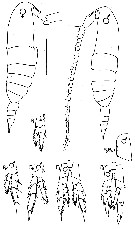
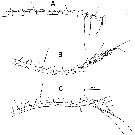
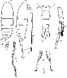 Issued from : M.S. Kos in Field guide for plankton. Zool Institute USSR Acad., Vol. II, 1976. After Brodsky, 1950. Female: 1-2, habitus (dorsal and lateral, respectively); Male: 3, abdomen (dorsal); r, left P5; 4-5, denticles along inner edge of coxopodite of P5.
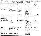
| | | | | Compl. Ref.: | | | Jaschnov, 1958 (p.838, fig.2); Fleminger, 1967 a (tabl.1); Heinrich, 1968 (p.287, fig.1, 3); McAllister, 1969 (p.199, , 218: Appendix 1, ingestion rate); Omori, 1969 (p.5, Table 1); jaschnov, 1970 (p.205, chart); Frost, 1972 (p.805, feeding behavior); Fager, 1973 (p.297, table 1, mortality coefficient); Sargent & Lee, 1975 (p.15, lipid synthesis); Mullin & al., 1975 (p.259, ingestion vs. food concentration); Frost, 1975 (p.263, feeding behavior); Griffiths & Frost, 1976 (p.1, chemical communication/aesthetes); Mullin & Brooks, 1976 (p.784, distributional heterogrneity vs. nutrition-respiration, comparison pump vs. net-haul); Gibson & Grice, 1977 (p.85, Table 1, copper pollution); Frost, 1977 (p.472, feeding behavior); Enright, 1977 (p.856, diurnal vertical migration vs. metabolic model); Enright & Honegger, 1977 (p.873, diurnal vertical migration vs. metabolic advantages); Fernandez, 1979 (p.313, nauplius feeding); Vidal, 1980 (p.111, size, growth vs. environmental factors); 1980 a (p.135, development & molting rates); 1980 b (p.195, metabolism); 1980 c (p.203, production); Runge, 1980 (p.134, feeding behaviour); Poulet & Marsot, 1980 (p.198, Table 1, 2, feeding); Landry, 1980 (p.545, prey detection-A1); 1980 a (p.135); Holliday & Pieper, 1980 (p.136, Rem.: acoustic data); Cox & Willason, 1981 (p.307, enzyme); Landry, 1981 (p.77, herbivory vs. carnivory); Star & Mullin, 1981 (p.1322, abundance); Landry, 1981 (p.77, predation); Cox & al., 1982 (p.1127, Rem.: p.1149); Huntley, 1982 (p.81, filtration rate vs. food); Harris, 1982 (p.71, feeding behaviour vs. particle-size spectrum); Hassett & Landry, 1982 (p.211, digestive carbohydrase activities); 1983 (p.47, feeding, digestive enzyme activities); Jacoby & Youngbluth, 1983 (p.84, Table 4, Rem: mating); Landry, 1983 (p.614, development times vs. stages); Huntley & al., 1983 (p.151, nutrition, faecal pellets production); Runge, 1984 (p.53, egg production); Pieper & Holliday, 1984 (p.226, Table 1, Figs.3, 7, 8); Hakanson, 1984 (p.794, feeding vs. lipids); Miller & al., 1984 (p.1274, molting rates); Kleppel & Pieper, 1984 (p.193, gut contents); Miller C.A. & Landry, 1984 (p.265, ingestion, excretion); Landry & al., 1984 (p.361, assimilation); Allredge & al., 1984 (p.75, aggregation); Jacobsen & Azam, 1984 (p.495, fecal pellet/bacteria); Runge, 1984 (p.125, egg production); 1985 (p.382, egg production); Downs & Lorenzen, 1985 (p.1024, fecal pellets, C: phaeopigment ratio); Kawamura & Hirano, 1985 (p.626, Table 1, fig.3, horizontal distribution); Mullin & al., 1985 (p.151, Appendix: as ''Calanus'', vertical structure vs. storm & larval fish effects); Frost, 1985 (p.1, food limitation); Gordon & al., 1985 (p.89, Table 3, fish diet); Downs & Enzeroth, 1985 (p.553, fecal pellet); Ayukai & Nishizawa, 1986 (p.3, egestion rate vs ingestion rate); Brinton & al., 1986 (p.228, Table 1); Mackas & Anderson, 1986 (p.115, Table 2); Mackas & Burns, 1986 (p.383, feeding); Huntley & a., 1986 (p.105, rejected prey); Marin & al., 1986 (p.49, feeding rates); Ayukai, 1987 a (p.585, 586, Rem.: feeding); Sykes & Huntley, 1987 (p.19, feeding behavior); Huntley & al., 1987 (p.911, grazing); Hakanson, 1987 (p.881, lipid content); Mobley, 1987 (p.199, ingestion rate); Huntley, 1988 (p.83, Table 1, feeding history); Donaghay, 1988 (p.469, acclimatation v.s. food quality & trophic dominance); Hassett & Landry, 1988 (p.63, feeding); Mullin, 1988 (p.291, nauplius production & distribution, variability); Jimenez-Perez & Lara-Lara, 1988 (p.122); Kleppel & al., 1988 (p.231, feeding); Lopez M. & al., 1988 (p.715, gut pigments); McLaren & al., 1988 (p.275, DNA content, development rate: egg-nauplius); Frost, 1988 (p.675, vertical migration); Wiebe & al., 1988 (tab.7); Dey & al., 1988 (p.321, 323, UV-B effect); Ohman, 1988 (p.143, Table 1: lipid content); Landry & Fagerness, 1988 (p.509, fig.3: clearance rate, Table 3, 4, 5, 6, figs. 4, 6, 8); Hernandez-Trujillo, 1989 a (tab.1); Bollens & Frost, 1989 a (p.1072, vertical migration vs.predators); Dagg & al., 1989 (p.1062, diel migration, feeding); Cervantes-Duarte & Hernandez-Trujillo, 1989 (tab.3); Penry & Frost, 1990 (p.1207, fig.1, ingestion rates); Hassett & Landry, 1990 (p.991, diet & starvation vs digestive enzyme activity); Cervantes-Duarte & Hernandez-Trujillo, 1991 (1993) (tab.I); Razouls S. & al., 1991 (p.65, developpement /sexual maturity); Hattori, 1991 (tab.1, Appendix); Shih & Marhue, 1991 (tab.2, 3); Mullin, 1991 (p.65, eggg production); 1991 a (p.1381, reproduction & mortality variability); 1991 b (p.165, 180, fig.7.10- 7.13, egg production, biomass & secondary production); Lopez M. & al., 1991 (p.79, development time); Huntley & Lopez, 1992 (p.201, Table A1, B1, egg-adult weight, temperature-dependent production, growth rate); Cary & al., 1992 (p.404, artificial food-microcapsule); Kimmerer, 1993 (tab.2); Dagg, 1993 (p.163, Table 1, abundance); Bollens & al., 1993 (p.1827, vertical distribution vs. predators); Landry & al., 1994 (p.55, abundance, grazing); Landry & al., 1994 a (p.73, grazing, gut evacuation); Osgood & Frost, 1994 (p.627, life history, vertical migration); 1994 a (p.13, ontogenic vertical migration); de Angelis & Lee, 1994 (p.1298, methane production); Mullin, 1994 (p.142, distribution & reproduction: ''annual anomaly''); 1995 (p.175, Californian El Niño effect); Palomares Garcia & Vera, 1995 (tab.1); Shih & Young, 1995 (p.68); Trujillo-Ortiz, 1995 (p.2175, cohort analysis); Juhl & al., 1996 (p.1198, pigments/diets); Uye, 1996 (p.89, egg production); Cowie & Hedges, 1996 (p.581, digestion efficiencies); Kotani & al., 1996 (tab.2); Dower & Mackas, 1996 (p.837, seamount effects vs. abundance); Ban S, Burns C. & al., 1997 (p.287, fig.1, Table 1, 2, feeding, reproduction); Mullin, 1998 (p.115, Rem.: interdecadal variation); Mauchline, 1998 (tab.15, 18, 19, 21, 22, 24, 38, 45, 46, 47, 48, 51, 58, 62, 63, 64, fig.72); Ban & al., 1998 (p.42, abundance vs. phytoplankton bloom); Suarez-Morales & Gasca, 1998 a (p108); Ohman & al., 1998 (p.1709, organic composition, vertical distribution, ETS activity, egg production, dormancy: Table 3); Gomez-Gutiérrez & Peterson, 1999 (p.637, Table I, II, III, VI, figs.4, 5, 6, 7, abundance, egg production); Hernandez-Trujillo, 1999 (p.284, tab.1); 1999 a (p.154); Lavaniegos & Gonzalez-Navarro, 1999 (p.239, Appx.1); Dolganova & al., 1999 (p.13, tab.1); Mackas & Tsuda, 1999 (p.335, Table 1); Huggett & Richardson, 2000 (p.1843, tab.2); Pinchuk & Paul, 2000 (p.4, table 1, % occurrence); White & McLaren, 2000 (p.751, tab.1); Haury & al., 2000 (p.69, Table 1); Lenz & al., 2000 (p.338); Rebstock, 2001 (tab.2, 4); 2002 (p.71, Table 3, 5, 6, Figs.2, 3: climatic variability); Peterson & al., 2002 (p.353); Peterson & al. 2002 (p.381, Table 2, fig.6, interannual abundance); Yamaguchi & al., 2002 (p.1007, tab.1); Hernandez-Trujillo & Suarez-Morales, 2002 (p.748, tab.1); Peterson & Keister, 2003 (p.2499, interannual variability); Keister & Peterson, 2003 (p.341, Table 1, 2, abundance, cluster species vs hydrological events); Rau & al., 2003 (p.2431, N variations vs climate variability 1950-2000); Park, W & al., 2004 (p.464, tab.1); Zuenko & Nadtochii, 2004 (p.526, tab.1); Mackas & al., 2004 (p.875, Table 2); Ashjian & al., 2005 (p.1380: tab.2); Mackas & al., 2005 (p.1011, tab.2); Pierson & al., 2005 (p.349, vertical distribution vs. Chl a concentration); Miller C.B., 2005 (p.136, clearance vs factors, p.140, fig.7.7, ingestion rate vs. body weight, stages; p.149: growth rates, figs.7.12, 7.13, 7.14), 7.16); Frangoulis & al., 2005 (p.254, Table I: C/N/P fecal pellet composition); Lopez-Ibarra & Palomares-Garcia, 2006 (p.63, Tabl. 1, seasonal abundance vs El-Niño, Rem.: p.67, 71, 73); Ware & McQueen, 2006 (p.28, Table B1, weight ranges); Lavaniegos & Jiménez-Pérez, 2006 (p.136, tab.2, 3, Rem); Hooff & Peterson 2006 (p.2610); C.L. Johnson, 2007 (p.203, dormant stage V); Zirbel & al., 2007 (p.106, egg development); Humphrey, 2008 (p.83: Appendix A); Liu & Hopcroft, 2008 (p.930: fig.7); Kobari & al., 2008 (p.1648, coppodids I-VI, depth distribution); Ohman & Hsieh, 2008 (p.359, mortality vs spatial); Takahashi & al., 2008 (p.222, Table 2, grazing impact); Galbraith, 2009 (pers. comm.); Chiba & al., 2009 (p.1846, Table 1, occurrence vs temperature change); Hernandez-Trujillo & al., 2010 (p.913, Table 2); W.-B. Chang & al., 2010 (p.735, Table 2, abundance); Bollens & al., 2011 (p.1358, Table III); Batten & Walne, 2011 (p.1643, Table I, abundance vs temperature interannual variability); Homma & al., 2011 (p.29, Table 2, 3, abundance, feeding pattern: suspension feeders); Keister & al., 2011 (p.2498, interannual variation); DiBacco & al., 2012 (p.483, Table S1, ballast water transport); Ohman & al., 2012 (p.46, N variations as index of climate variations over 54-year time period); Lavaniegos & al., 2012 (p. 11, Table 1, fig.3, seasonal abundance, Appendix); Karaköylü & Franks, 2012 (p.55, grazing); Takahashi M. & al., 2012 (p.393, Table 2, water type index); Palomares-Garcia & al., 2013 (p.1009, Table I, fig.7, abundance vs environmental factors); in CalCOFI regional list (MDO, Nov. 2013; M. Ohman, pers. comm.); Kobari & al., 2013 (p.78, Table 2); Mendoza Portillo, 2013 (p.37: Fig.7, seasonal dominance, p.42: fig.10, biomass); Peijnenburg & Goetze, 2013 (p.2765, genetic data); Batchelder & al., 2013 (p.34, Rem.: p.42, 44); Pierson & al., 2013 (p.49, vertical migration vs seasonal environment); Barton & al., 2013 (p.522, Table 1: metabolism, diapause, population dynamic, feeding mode, biogeo); Chiba S. & al., 2015 (p.968, Table 1: length vs climate); Ohtsuka & Nishida, 2017 (p.565, Table 22.1); Baumgartner & Tarrant, 2017 (p.387, Table 1, diapause); Record & al., 2018 (p.2238, Table 1: diapause); Palomares-Garcia & al., 2018 (p.178, Table 1: occurrence) | | | | NZ: | 6 + 1 doubtful | | |
|
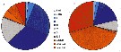
Distribution map of Calanus pacificus by geographical zones
|
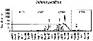
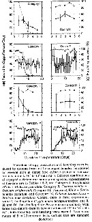
| | | | | | 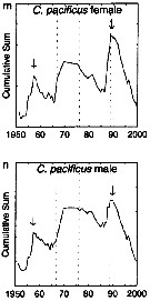 issued from : G.A. Rebstock in Global change Biology, 2002, 8. [p.77, Fig.2 m, n]. issued from : G.A. Rebstock in Global change Biology, 2002, 8. [p.77, Fig.2 m, n].
Climatic regime shifts and decadal-scale variability in calanoid copepod populations off southern California (31°-35°N, 117°-122°W.
Cumulative sums of nonseasonal anomalies from the long-term means of copepod abundance from years 1950 to 2000.
A negative slope indicates a period of below-average anomalies; a positive slope indicates a period of above-average anomalies. Abrupt changes in slope indicate step changes. Step changes are marked with arrows (upward-pointing for increases).
The October 1966 cruise (prior to the increase in sampling depth), March 1976 cruise (prior to the 1976-77 climatic regime shift), and October 1988 cruise (prior to the hypothesized 1989 climatic regime shift) are marked with vertical lines. |
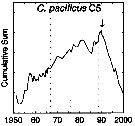 issued from : G.A. Rebstock in Global change Biology, 2002, 8. [p.77, Fig.2 o]. issued from : G.A. Rebstock in Global change Biology, 2002, 8. [p.77, Fig.2 o].
Climatic regime shifts and decadal-scale variability in calanoid copepod populations off southern California (31°-35°N, 117°-122°W.
Cumulative sums of nonseasonal anomalies from the long-term means of copepod abundance from years 1950 to 2000.
A negative slope indicates a period of below-average anomalies; a positive slope indicates a period of above-average anomalies. Abrupt changes in slope indicate step changes. Step changes are marked with arrow (upward-pointing for increases).
The October 1966 cruise (prior to the increase in sampling depth), March 1976 cruise (prior to the 1976-77 climatic regime shift), and October 1988 cruise (prior to the hypothesized 1989 climatic regime shift) are marked with vertical lines. |
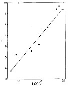 issued from : B.W. Frost in Limnol. Oceanogr., 1977, 22 (3). [p.473, Fig.1]. issued from : B.W. Frost in Limnol. Oceanogr., 1977, 22 (3). [p.473, Fig.1].
Relationship between maximum clearance rate F (ml /copepod /day) for adult females of Calanus pacificus and size of food particle (measured as log V, where V is mean cell volume in micro m3).
All measurements of clearance rate made at food concentrations below critical concentration.
Line, fitted by least-squares linear refression: F = 2.43 (log V) - 3.92; r = 0.73, N = 143. Significant linear relationship also exists between F and mean cell diameter (micrometre). |
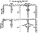
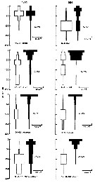 issued from : S.M. Bollens & B.W. Frost inLimnol. Oceanogr., 1989, 34 (6). [p.1078, Fig.2]. issued from : S.M. Bollens & B.W. Frost inLimnol. Oceanogr., 1989, 34 (6). [p.1078, Fig.2].
Vertical distribution of adults females of Calanus pacificus in Dabob Bay (Washinton State) in 1985 and 1986.
For each set of dates, day (clear) and night (black) vertical distributions are means of four vertical series of samples collected in pairs near noon and midnight on each of two consecutive days.
Numbers in italics are vaues of V = dependence of the strenth of the diel vertical migration exhibited by C. pacificus on the abundance of planktivorous fish actively feeding on C. pacificus in the surface 50 m of the water column |
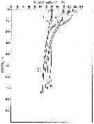
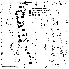
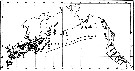 issued from : W.A. Jaschnov in Int. Revue ges. Hydrobiol., 1970, 55 (2). [p.206, Fig.4] issued from : W.A. Jaschnov in Int. Revue ges. Hydrobiol., 1970, 55 (2). [p.206, Fig.4]
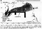
Distribution of Calanus pacificus from literary sources (as C. finmarchicus or C. helgolandicus) and unpublished data (black circles).
Solid line indicates the southern boundary of the distribution of the species. Arrows denote some of the currents.
Nota: After Jaschnov (1970, p.205 & following) it seems highly probable that the centre of distribution of the subtropical species lies in the East China Sea and Yellow Seas, where it occurs in large quantities. The species does not occur in the tropical and subtropical waters of the Pacific Ocean nor in the southern part of the Kuroshio Current.
The main flow of the Kuroshio divides at the latitude of Tokara Strait. Large masses of water from the Yellow Sea also flow into the Japan Sea. The area of intense mixing of these waters lies to the west of Kyushyu.
The Tsushima Current brings into the Japan Sea many tropical and subtropical plankton forms (see in Nishimura, 1965). C. pacificus , too, is brought by this current from the Yellow Sea to the Japan Sea, which may be considered as an area of immigration. Its distribution is closely associated with the Tsushima Current. It is known that the greater part of the water of this current (about 70 % on the average) runs into the Pacific Ocean through the Tsugaru Strait; the rest of the water flows into the Pacific through La Pérouse Strait.
The range of the species in the Pacific Ocean is closely associated with the subarctic surface waters. The zone of great concentrations of this species extending from the Tsugaru Strait in a northern direction is situated more to the north than the dynamic axis of the Kuroshio. With the waters of the Tsugura Current, running close to the eastern coast of Honshu, the species is carried southward along the coasts of Japan down to Kyusyu. C. pacificus is not encountered in the Kuroshio proper; this does not disagree with the findings of this species southeastward of Honshu, because they are reported from deeper layers underlying the waters of the Kuroshio and containing submerged Oyashio water (see Omori, 1967).
This species penetrates into the southern part of the Bering Sea with the waters of the warm current. At present it is hard to decide whether the population inhabiting the Gulf of Alaska is of local origin or its maintenance depends on an inflow of new populations from the wester regions of the ocean. |
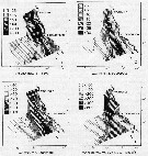 issued from : J.L. Hakanson in Limnol. Oceanogr., 1987, 32 (4). [p.883, Fig. 1 (partial)]. Results of a field sampling programm covered the California Current between Los Angeles and San Francisco in April 1984 (CalCOFI, cruise 8404) in order to determine the feeding condition of Calanus pacificus copepodite V. issued from : J.L. Hakanson in Limnol. Oceanogr., 1987, 32 (4). [p.883, Fig. 1 (partial)]. Results of a field sampling programm covered the California Current between Los Angeles and San Francisco in April 1984 (CalCOFI, cruise 8404) in order to determine the feeding condition of Calanus pacificus copepodite V.
B: Distribution of total Chl a. C: Distribution of mean wax ester content in C. pacificus . E: Distribution of mean dry weight in C. pacificus; F: Distribution of macrozooplankton volume (excluding organisms > 5 ml) from Bongo net (mesh aperture = 505 micrometers), towed obliquely from 210 m to the surface. |
 issued from : R.P. Harris in J. mar. biol. Ass. U.K., 1982, 62. [p.83, Figs. 10, 11]. issued from : R.P. Harris in J. mar. biol. Ass. U.K., 1982, 62. [p.83, Figs. 10, 11].
Comparison of the feeding behaviour of Calanus pacificus (large species) and Pseudocalanus minutus (small species) in two controlled experimental ecosystems (CEEs) with phytoplankton food (CEE 2: mainly diatoms; CEE 3: mainly flagellate population).
Fig.10: A, Mean clearance rate related to particle size. All experiments included. C. pacificus: black circle; P. minutus: open circle. CEE 2: line; CEE 3: dotted line.
Fig. 11: B, Comparison of mean retention efficiencies in relation to particle size. mean value for all experiments days, both CEEs combined.
C. pacificus: black circle; P. minutus: open circle.
Nota: In the fig.10 (A) the large decrease in C. pacificus clearance rate for the highest size channel may represent decreased ability to ''handle'' these large paricles. The Fig.11 (B) demontrates that below 20 micrometers P. minutus characterizing a small form) filters with a greater efficiency in all size channels. Between 20 and 70 micrometers the converse is observed with C. pacificus (characterizing a large form) having greater efficiency.
For the authors, it was found over a series of experiments lasting 72 days, during which a wide range of phytoplankton was encountered, that on average fed on slightly larger particles (1.2 x diameter) than Pseudocalanus. However, despite the large difference in body size (x 10 dry weight) there was evidence that on most occasions both species were competing for the same food resource over a wide range of the particle-size spectrum. |
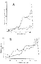
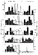
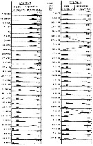 issued from : M.M. Mullin & E.R. Brooks in Limnol. Oceanogr., 1967, 12. [p.660, Fig.2]. issued from : M.M. Mullin & E.R. Brooks in Limnol. Oceanogr., 1967, 12. [p.660, Fig.2].
Relative abundance of the developmental stages of Calanus pacificus ar various times over at 2-yr period in the California Current, a few kilometers offshore from Scripps Institution of Oceanography (La Jolla, San Diego)
The number associated which each histogram shows the total number of individuals of all stages of that species caught with net in a 90-m vertical tow.
The height of the shaded bar associated with each developmental stage shows the relative contribution of that stage to this total. If less than 10 individuals were found in the samples from any date, no histogram was drawn. Before 23 March 1965, no nauplii were sampled, so frequencies are based on copepodite stages only. Diagonal lines connect supposed generations.
Nota : Mullin & Brooks indicate that the local species breed more or less contibuously so that the population is dominated by the naupliar stages during most of the year. Only occasionally (as between 12 April and 10 May or between 24 August and 20 September 1966) was there an indication of a discrete generation maturing and producing offspring. These ibdications suggest a generation time of about 4 weeks, but this interpretation is questionable because the simultaneous occurrence of juveniles with older copepodites that are neither their parents nor their siblings seems likely. Table 1 (from culture in the laboratory) shows the time required to attain various developmental stages. In general, the males molted from the immature condition to the adult stage somewhat before the females and also died off sooner than the females.
Concerning the fecundity, Mullin & Brooks indicate under ideal conditions, the total number of eggs produced by wild females believed to have copulated only a short time before capture (many were still carrying spermatophores). For two groups of 15 females, each gave means of 613 and 691 eggs) female over 9 weeks. This is somewhat higher than the egg production reported for Calanus helgolandicus by Marshall & Orr (1955). These estimates must be considered minimal because some of the females used may have laid eggs before capture or other causes. |
 issued from : M.M. Mullin & E.R. Brooks in Limnol. Oceanogr., 1967, 12. [p.658, Fig.1]. issued from : M.M. Mullin & E.R. Brooks in Limnol. Oceanogr., 1967, 12. [p.658, Fig.1].
Vertical distribution of temperature at the sampling station in the California Current, a few kilometers offshore from Scripps Institution of Oceanography (La Jolla, San Diego) in various months (indicated by roman numerals). |
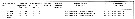
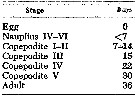 issued from : M.M. Mullin & E.R. Brooks in Limnol. Oceanogr., 1967, 12. [p.659, Table 1]. issued from : M.M. Mullin & E.R. Brooks in Limnol. Oceanogr., 1967, 12. [p.659, Table 1].
Approximate cumulative time (in days) required for development at 12°C in the laboratory based on three stocks of Calanus pacificus. |
 Issued from : M.E. Huntlley, K.-G. Barthel & J.L. Star in Mar. Biol., 1983, 74. [p.155, Fig.7]. Issued from : M.E. Huntlley, K.-G. Barthel & J.L. Star in Mar. Biol., 1983, 74. [p.155, Fig.7].
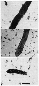
Calanus pacificus from la Jolla (California). Photomicrographs of faecal pellets produced by CIV copepodites feeding on (a) mixture of the diatom Thalassiosira weissflogii cells (13.1 µm Equivalent Sperical Diameter) and large beads; (b): cells alone; (c): large beads alone.
Scale bar = 125 µm.
Nota: When offered mixtures of cells and polysttyrene of two sizes (11.1 and 16.5 µm ESD)beads, the filtration and ingestion rates were significantly greater on the cells than on the beads, irrespective of bead size.
the species demonstrates a clear preference for Gyrodinium dorsum (27 µm) relative to Peridinium trochoideum (22µm), two dinoflagellates).
The results cannot be explained by a model of passive, size-selective feeding.
|
 issued from : M.J. Dagg, B.W. Frost & W.E. Walser, Jr. in Limnol. Oceanogr., 1989, 34 (6). [p.1065, Fig.1]. issued from : M.J. Dagg, B.W. Frost & W.E. Walser, Jr. in Limnol. Oceanogr., 1989, 34 (6). [p.1065, Fig.1].
Vertical distribution of adult females of Calanus pacificus, 6 and 7 May 1986, at Dabob Bay (47°45.5'N, 122°49.5'W).
Nota: Vertical distribution determined by vertical hauls with a multinet sampler (333-µm mesh). Water column sampled over six depth stata: 175-125, 125-75, 75-50, 50-25, 25-10, and 10-0 m. |
 Issued from : E. Brinton, A. Fleminger & D. Siegel-Causey in CalCOFI Rep., 1986, 27. [p.262, Fig.23]. Issued from : E. Brinton, A. Fleminger & D. Siegel-Causey in CalCOFI Rep., 1986, 27. [p.262, Fig.23].
Roughly estimated abundance of Calanus pacificus californicus in the 0-140 m layer sampled by CalCOFI during April and August 1957 in the Gulf of California. |
 Issued from : M.J. Zirbel, C.B. Miller & H.P. Batchelder in Limnol. Oceanogr.: Methods, 2007, 5. [p.109, Fig.4]. Issued from : M.J. Zirbel, C.B. Miller & H.P. Batchelder in Limnol. Oceanogr.: Methods, 2007, 5. [p.109, Fig.4].
Approximate observed development stage durations for Calanus pacificus eggs from Dabob Bay (Washington), at 10-12°C, based on 72 clutches divided into groups of > 10 eggs and variously assigned to killing times..
|
 Issued from : M.J. Zirbel, C.B. Miller & H.P. Batchelder in Limnol. Oceanogr.: Methods, 2007, 5. [p.109, Fig.6]. Issued from : M.J. Zirbel, C.B. Miller & H.P. Batchelder in Limnol. Oceanogr.: Methods, 2007, 5. [p.109, Fig.6].
Age proportions for eggs within 0-100 m of the water column for Calanus pacificus in Dabob Bay (Washington) at 07.00 hour on (A) 23 April 2003 and (B) 24 April 2003.
Eggs (n > 200 for each profile were collected, sorted, stained, and assayed for development stage as described on figure. |
 Issued from : W.T. Peterson, J.E. Keister & L.R. Feinberg in Prog. Oceanogr., 2002, 54. [p.390, Fig.6]. Issued from : W.T. Peterson, J.E. Keister & L.R. Feinberg in Prog. Oceanogr., 2002, 54. [p.390, Fig.6].
Abundance (number per cubic meter) of C. marshallae at the station NH5 (off Newport, Oregon, at depth 30 m) from May 1996 through September 1999.
Compare the occurrences between this species and C. marshallae correlatd with the effects of the 1997-98 El Niño effect on the hydrography off the central Oregon coast.. |
 Issued from : T. Yoshiki, B. Yamanoha, T. Kikuchi, A. Shimizu & T. Toda in Mar. Biol., 2008, 156. [p.104, Table 4]. Issued from : T. Yoshiki, B. Yamanoha, T. Kikuchi, A. Shimizu & T. Toda in Mar. Biol., 2008, 156. [p.104, Table 4].
Egg development time and egg sinking rate of three Calanus species. |
 Issued from : M.D. Ohman, A.V. Drits, M.E. Clarke & S. Plourde in Deep-Sea Res. II, , 1998 , 45. [p.1719, Fig. 4 C]. Issued from : M.D. Ohman, A.V. Drits, M.E. Clarke & S. Plourde in Deep-Sea Res. II, , 1998 , 45. [p.1719, Fig. 4 C].
Vertical distribution of copepod in the San Diego Trough in June and December. Adult female and copepodid stage V of Calanus pacificus californicus.
Dark symbols illustrate nightime distributions, open symbols illustrate daytime distributions, each plotted at the mid-point of the sampling interval. Sampling extended deeper in December than in June.
Sampling out in the San Diego Trough (near 32°50'N, 117°40'W) in 6-14 June 1992 and 15-22 December 1992.
The species does not exhibit a pattern of winter dormancy - i.e. , synchronous developmental arrest as copepodid stage V, descent into deep waters, reduced metabolism, and lack of winter reproduction. Calanus pacificus californicus has a biphasic life history in this region, with an actively reproducting segment of the population in surface waters overlying a deep dormant segment in winter. In Dabob Bay (47°45'N), the subspecies exhibits a dormancy response; copepodid V's accumulate and dominate the stage structure of the population during autumn-winter, most of which remain in deeper water day and night in October and February. Egg production by females does not begin in this locality until March. |
 Issued from : M.D. Ohman, A.V. Drits, M.E. Clarke & S. Plourde in Deep-Sea Res. II, , 1998 , 45. [p.1730, Table 3]. Issued from : M.D. Ohman, A.V. Drits, M.E. Clarke & S. Plourde in Deep-Sea Res. II, , 1998 , 45. [p.1730, Table 3].
Differential dormancy of co-occuring copepods in the California Current System in the San Diego Trough.
Indices used to differentiate actively growing from dormant animals included developmental stage structure and vertical distribution; activity of aerobic metabolic enzymes (Citrate Synthase and Electron Transfer System complex); investment in depot lipids (wax esters and triacylglycerols); in situ grazing activity from gut fluorescence, and egg production rates. |
 Issued from : A. Bucklin & T.C. Lajeunesse in CalCOFI, 1994, 35. [p.46, Fig.1]. Issued from : A. Bucklin & T.C. Lajeunesse in CalCOFI, 1994, 35. [p.46, Fig.1].
Geographic distribution of the subspecies of Calanus pacificus.
Nota: C. pacificus may include sveral subspecies, although no morphological characters diagnostic of each subspecies have been found.
The authors use DNA sequence variation of a miyochondrial gene to investigate the degree of genetic differentiation associated with these systemating groupings and to begin a study of the evolutionary significance of geographic variation in the species.
The DNA sequence of a 449 base pair portion of the mitochondrial 16S rRNA gene was determined for 27 individuals collected from five sites in the North Pacific Ocean..
The molecular genetic differentiation between individuals of C. p. oceanicus and C. p. californicus (0.9% to 1.0% sequance difference) was greater than that between individuals of C. p. californicus from different geographic region (0.2% to 0.5% difference), but less than that among species of Calanus (12% to 18% difference).
The strongest evidence of subspecies differentiation is that the C. p. oceanicus individuals were grouped together and separate from C. p. californicus on a tree constructed by neighbor joining wiyj 1000 bootstrapped subrepkicates. |
 Issued from : A. Bucklin & T.C. Lajeunesse in CalCOFI, 1994, 35. [p.49, Fig.4]. Issued from : A. Bucklin & T.C. Lajeunesse in CalCOFI, 1994, 35. [p.49, Fig.4].
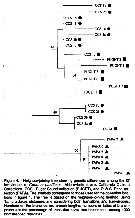
Neighbor-joining tree showing genetic differences among the 27 individuals of calanus pacificus.
The Ocean Weather Station Papa (PAPA): 50°N, 145°W.
CCS1: California Current (in June 1992).
CCS2: California Cooperative Fisheries Investigation (CalCOFI) surveys in November 1989.
CCS3: 32°25"N, 118°10'W,
Puget Sound (PUGET): 47°45.5'N, 122°49.5'W. in April 1992. |
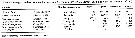
 Issued from : H. Saito & A. Tsuda in Deep-Sea Res. I, 47. [p.2146, Table I]. Issued from : H. Saito & A. Tsuda in Deep-Sea Res. I, 47. [p.2146, Table I].
Egg diameter and prosome length (PL) of females of Calanus pacificus after McLaren & al., 1988,
Nota: Compare with N. cristatus, N. tonsus and N. flemingeri, and others species in genus Calanus. |
 Issued from : C.J. Corkett, I.A. McLaren & J.-M. Sevigny in Syllogeus, 1986, 58. [p.545, Table I]. Issued from : C.J. Corkett, I.A. McLaren & J.-M. Sevigny in Syllogeus, 1986, 58. [p.545, Table I].
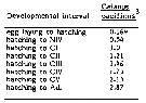
Relative times to reach various stages of C. pacificus, assuming equiproportional development.
All times expressed relative to time between hatching and molting to CI.
3 : From Landry (1983, Table 2), who gives stage durations at 15°C..
Nota: Compare with Calanus hyperboreus, C. finmarchicus , C. helgolandicus and C. glacialis. |
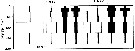
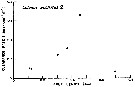
 Issued from : C.B. Miller in Biological Oceanography, 2005. Blackwell Publishing. [p.140, Fig.7.7]. After Paffenhöfer, 1971. Issued from : C.B. Miller in Biological Oceanography, 2005. Blackwell Publishing. [p.140, Fig.7.7]. After Paffenhöfer, 1971.
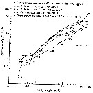
Ingestion rate of Calanus pacificus as a function of body weight.
Filtering rates increase similarly. Naupliar and copepodid stages, indicated by Roman numerals, varied somewhat in weights attained and ingestion rates among four species of food, represented by separate lines.
Ingestion increases roughly as weight to the 0.87 power. |
 Issued from : C.B. Miller in Biological Oceanography 2004/2005, Blackwell Publishing. [p.157, Table 7.1]. After Mullin & Brooks, 1970. Issued from : C.B. Miller in Biological Oceanography 2004/2005, Blackwell Publishing. [p.157, Table 7.1]. After Mullin & Brooks, 1970.
Calanus pacificus dominant zooplankters in the California Current. Data characterize the season of peak production. Mostly taken from Landry (1978): 41 mgC m-2 day-1.
Miller underlines the difficulties of the production estimations for single species, and virtually none for whole systems, but we would like to know how much food the oceans produces for animals we harvest like herring, anchovy, cod, and pollack. See Huntley & Lopez, 1992: model); Kleppel, Davis & Carter, 1996; Huntley, 1996; Hirst & Sheader, 1997; Hirst & Lampitt, 1998; Vidal, 1980. |
 Issued from : C.B. Miller in Biological Oceanography 2004/2005, Blackwell Publishing. [p.166, Fig.8.6]. After Uye, 1996. Issued from : C.B. Miller in Biological Oceanography 2004/2005, Blackwell Publishing. [p.166, Fig.8.6]. After Uye, 1996.
Egg production rate (bar height) and egg viability (black = healthy nauplii; hatched = deformed nauplii; white = non-viable, no hatching) of Calanus pacificus.
Females were initially fed Prorocentrum minimum (a dinoflagellate), then switched to the diatom Chaetoceros difficilis, on day 2, then switched back to Prorocentrum on day 11 (as indicated by arrows along the top.
Fecal pellet production (connected circles) indicates feeding levels.
Miller (p.165) underlines that females collected off the Oregon coast, fed alternately with several different diatoms and with several dunoflagellates. Females eating diatoms soon spawn eggs that don't develop. Switched to dinoflagellates the viability of their eggs recovers. Nauplii that do hatch from diatom-fed females are often teratogenized, they are a sad sight. See Miralto & al. (1999). |
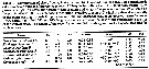
 Issued from : S. Ban, C. Burns, J. Castel, Y. Chaudron & al. in Mar. Ecol. Prog. Ser., 1997, 157. [p.289, Table 1]. Issued from : S. Ban, C. Burns, J. Castel, Y. Chaudron & al. in Mar. Ecol. Prog. Ser., 1997, 157. [p.289, Table 1].
Synopsis of feeding/reproduction experiments. A total of 17 diatom and 16 copepod species, representative of a variety of worldwide temperate and subarctic environments (E: estuarine, C: coastal ocean), were screened.
Data for fecundity and hatching success are average values measured at the start and end of the inciubations in a minimum of 3 replicate batches, showing the variation in time of the effects of diatoms on copepod reproduction.
Level of significance of the diatom effect between treatments and controls (e.g. non-diatom diets) in categories I to III was p < 0.01. No.. rank (for comparison with Table 2, p.290).
For the signification of the categories I to IV (fecundity vs. Hatching success vs. Duration of experiment days-1): See Eurytemora affinis, Calanus pacificus, Calanus finmarchicus, Temora stylifera.
List of the 12 marine or estuarine species studied (fresh water excluded. CR): Acartia clausi, A. grani, A. steueri, A. tonsa, Calanus finmarchicus, C. helgolandicus, C. pacificus, Centropages hamatus, C. typicus, Eurytemora affinis, Temora longicornis, T. stylifera. |
 Issued from : S. Ban, C. Burns, J. Castel, Y. Chaudron & al. in Mar. Ecol. Prog. Ser., 1997, 157. [p.288, Fig. 1]. Issued from : S. Ban, C. Burns, J. Castel, Y. Chaudron & al. in Mar. Ecol. Prog. Ser., 1997, 157. [p.288, Fig. 1].
Variations of egg production and hatching rates induced by diatoms ingested by copepod females maintained for several days in dense food cultures. Selected combinations of the data sets in Table 1 & 2. For categories in function of the duration of experiments (days). |
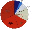
 Issued from : G.A. Lopez-Ibarra & R. Palomares-Garcia in Rev. Biol. Mar. Oceanogr., 2006, 41 (1). [p.67, Figs. 3, 4]. Issued from : G.A. Lopez-Ibarra & R. Palomares-Garcia in Rev. Biol. Mar. Oceanogr., 2006, 41 (1). [p.67, Figs. 3, 4].
A (Fig.3): Sea surface temperature anomalies from January 1982 to September 1989 and May 1997 to December 1998 in Magdalena Bay (Baja California South, Mexico). After Palomares-Garcia & al., 2003.
B (Fig.4): Biogeographical affinity of the copepods community in Magdalena Bay in May 1997, August 1997, November 1997 and January 1998.
Nota: The aim is to study seasonal changes in copepods communities associated to environmental changes caused by El Niño 1997/1998, evaluated during the four most intensive months of the event. Among the copepods identified (66). In may, before the arrival of warm waters to the area, the taxocoenosis structure was characterized by a high dominance, low diversity and the predominance of 2 species of temperated affinity: Calanus pacificus and Labidocera trispinosa. During the warm period (August and November) the dominant species were tropical affinity: Acartia clausi and Acartia lilljeborgi. In August, diversity increased influenced by oceanic waters whereas in November, diversity increased in the entire bay; in January the dominance was relative low and the most abundant tropical species was Paracalanus aculeatus, and a general increase of the diversity was observed in the entire bay.
The most remarkable changes in the copepods community were coincident with the occurrence of positive temperature anomalies. Changes included a 75% increase of species of tropical affinity and the presence of Pontella fera and the replacement of the temperate species Paracalanus parvus, by Paracalanus aculeatus.
See abundance changes in Table 1. |
 Issued from : G.A. Lopez-Ibarra & R. Palomares-Garcia in Rev. Biol. Mar. Oceanogr., 2006, 41 (1). [p.68, Table 1 (part.)]. Issued from : G.A. Lopez-Ibarra & R. Palomares-Garcia in Rev. Biol. Mar. Oceanogr., 2006, 41 (1). [p.68, Table 1 (part.)].
Monthly average abundance of characteristic species in Magdalena Bay (Mexico) during El Niño 1997/1998.
Samples at 14 stations in the Magdalena Bay (South Baja California, Mexico) a lagoon system. At the border-line of the California Current where joining waters from the North, Central and Oriental Pacific.
Samples with a conical net (333 µm mesh aperture) drawing in surface. |
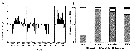
 Issued from : M.R. Landry & V.L. Fagerness in Bull. Mar. Sc., 1988, 43 (3) [p.512, Fig.3]. Issued from : M.R. Landry & V.L. Fagerness in Bull. Mar. Sc., 1988, 43 (3) [p.512, Fig.3].
Clearance rates of Calanus pacificus feeding on naupliar (closed circles) and copepodid stages (open circles).
Data from Landry (1980). |
 Issued from : M.R. Landry & V.L. Fagerness in Bull. Mar. Sc., 1988, 43 (3) [p.514, Table 2]. Issued from : M.R. Landry & V.L. Fagerness in Bull. Mar. Sc., 1988, 43 (3) [p.514, Table 2].
Comparison of the predatory potential of Calanus pacificus and Euchaeta elongata (= Paraeuchaeta elongata). Feeding rate estimates are for copepod eliciting maximum clearance rates.
Euchaeta data from Yen (1983; 1985); Calanus data from Landry (1980).
Population abundance estimates are for Dabob Bay, Washington during summer months (B. Frost, pers. comm.).
F = predatory clearance rates (volume swept clear of prey) see Landry, 1978.
F = V [Ln (nc) - ln (ne] / NT.
V = container volume (liters), N = number of predators, T = duration of the experiments (days), nc and ne are respectively, the numbers of intact (living) prey recovered from control and experimental containers. See also Frost, 1972.
For each of the predatory copepods, a preferred prey was defined as the prey for which calculated clearance rate was highest, i.e., F max. I max = maximum of prey captured for copepod by day. |
 Issued from : M.R. Landry & V.L. Fagerness in Bull. Mar. Sc., 1988, 43 (3) [p.514, Table 3]. Issued from : M.R. Landry & V.L. Fagerness in Bull. Mar. Sc., 1988, 43 (3) [p.514, Table 3].
Comparison of size of body and appendages for seven species of marine copepods. Relationships among predation rates, selection patterns, swimming speed and orientation, and morphology of prey sensory and capture appendages. |
 Issued from : M.R. Landry & V.L. Fagerness in Bull. Mar. Sc., 1988, 43 (3) [p.519, Fig. 8]. Issued from : M.R. Landry & V.L. Fagerness in Bull. Mar. Sc., 1988, 43 (3) [p.519, Fig. 8].
Swimming speeds and directions of the copepods Neocalanus cristatus, Euchaeta elongata (= Paraeuchaeta elongata), Calanus pacificus. See also to Tortanus discaudatus, Corycaeus anglicus, Oithona spinifera (= Oithona setigera).
Swimming speeds measured as displacement over 2-s time intervals. 0° is up.
Study of the relationships among predation rates, selection patterns, swimming speed and orientation, and morphology of prey sensory and capture appendages.
The mean relative swimming speeds (S) of the predatory copepods and their preferred prey were calculated by the equation (Gerritsen, 1980).
S = [u + v)3 - [u - v)3 / 6uv.
u and v are respectively, the mean swimming speeds (mm/s) of the prey and the predator. |
 Issued from : M.R. Landry & V.L. Fagerness in Bull. Mar. Sc., 1988, 43 (3) [p.522-523, Table 5]. Issued from : M.R. Landry & V.L. Fagerness in Bull. Mar. Sc., 1988, 43 (3) [p.522-523, Table 5].
Comparison of the predatory characteristics of seven planktonic marine copepods.
F max is the mean, maximum clearance rate measured for the predator feeding on its preferred prey. Prey are developmental stages of common species of planktonic copepods.
F = female, M = male, C5 = stage 5. |
 Issued from : M.R. Landry & V.L. Fagerness in Bull. Mar. Sc., 1988, 43 (3) [p.521, Table 4]. Issued from : M.R. Landry & V.L. Fagerness in Bull. Mar. Sc., 1988, 43 (3) [p.521, Table 4].
Mean horizontal (H) and vertical (V) components of swimming velocity for naupliar and copepodd I stages of Calanus pacificus.
Swimming speeds (mm/s) from 30-s video-recorded observations of N copepods.
See to Acartia clausii and Pseudocalanus sp. (as figured to P. elongatus for information, several species of this genus in the NE Pacific, see chart in zone 24). |
 Issued from : M.R. Landry & V.L. Fagerness in Bull. Mar. Sc., 1988, 43 (3) [p.525, Table 6]. Issued from : M.R. Landry & V.L. Fagerness in Bull. Mar. Sc., 1988, 43 (3) [p.525, Table 6].
Relationships between swimming speeds of predators and their preferred prey and ratios of maximum clearance rates for seven species of marine copepods. |
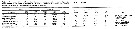
| | | | Loc: | | | Taiwan (S), China Seas (Yellow Sea), Japan Sea, Japan: Kuroshio region, Oyashio region, Hokkaido, Funka Bay, Honshu (Onagawa Bay), Kuril Is., S Okhotsk Sea, S Bering Sea, Alaska, S Aleutian, S Aleutian Basin, S Aleutian Is., Station "P", Cobb Seamount, Portland Inlet, British Columbia, Fjord system (Alice Arm & Hastings Arm), Hecate Strait, Vancouver Is., Puget Sound, Dabob Bay, off Washington coast, Francisco Bay, off N Hawaii, Oregon (off Newport), San Francisco Estuary, California, San Diego, Santa Monica Basin, off La Jolla (San Diego), Cobb Seamount, Baja California (Bahia Magdalena, W), G. of California (., Bahia de los Angeles), La Paz, Guaymas Basin, W Mexico | | | | N: | 182 | | | | Lg.: | | | (72) F: 3,01-2,62; M: 2,87-2,64; (131) F: 3,5-2,15; M: 3,1-2,35; (142) F: 3,1-2,6; M: 3,1-2,6; (145) F: 5,3-4,5; M: 4,4-4; (208) M: 2,7; (866) F: 2,7-3; M: 2,6-2,9; {F: 2,15-5,30; M: 2,35-4,40} (1259) F: 3,0;
The mean female size is 3.348 mm (n = 8; SD = 1.0543), and the mean male size is 3.062 mm (n = 9; SD = 0.6859). The size ratio (male : female) is 0.942 (n = 4; SD = 0.0567).
The greater size is gived by Esterly (1924) in the San Francisco Bay (145). Excepted this form, the mean female size is 2.830 mm (n = 6; SD = 0.4547) and the mean male size is 2.737 mm (n = 7; SD = 0.2434). The size ratio (male : female) is 0.967.
Chiba S. & al., 2015 (p.971, Table 1: Total length female (June-July) = 2.9 mm [optimal SST (°C) = 11.0].
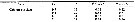
(1259) F: 3, 0 (total length), 2,3 (prosome length); A1 = 3,1 mm. (total length). | | | | Rem.: | Calanus pacificus californicus Brodsky, 1959 (F,M)
Syn.: C. finmarchicus : Esterly, 1924 (p.83, figs.F,M)
Ref.: Brodsky, 1962 a (p.1416); Kun, 1969 (p.997, figs.F, Rem.); Brodsky, 1972 (1975) (p.9, 82, 119, fig.); Brodsky & al., 1983 (p.170, figs.F,M, Rem.); Allredge & al., 1984 (p.75, aggregation); Fleminger, 1985 (p.275, 280, figs.F,M: A1, polymorphism); Bradford, 1988 (p.78); Bucklin & al., 1995 (p.658); Ohman & al., 1998 (p.1709, organic composition, vertical distribution, ETS activity, egg production, dormancy); Hill & al., 2001 (p.279, fig.2: phylogeny); Mackas & al., 2006 (L22S07, Table 2); Nuwer & al., 2008 (p.107, Rem.); Karaköylü & Franks, 2012 (p.55, grazing);
Loc.: California
Lg.: (131) F: 3,4-2,6; M: 2,75-2,56
For Ohman & al. (1998, p.1711), the analysis of mitochondrial DNA sequence variations confirms the subspecies (see in Bucklin & LaJeunesse, 1994).
Calanus pacificus japonicus Brodsky, 1959 (F,M)
Ref.: Brodsky, 1959 a (p.1545, figs.F,M); 1961 (p.16, figs.F,M); Vaupel-Klein, 1970 (p.7, Fig.M, tab.I & II: p.41, 42, F,M)
Loc.: Tartar Street, I. Sakhaline (coast), Amur Bay
Lg.: (339) F: 3,1-2,7; M: 2,8-2,6
Calanus pacificus oceanicus Brodsky, 1959 (F,M)
Syn.: no Calanus orientalis Jaschnov, 1975
Ref.: Brodsky, 1959 a (p.1545, figs.F,M); 1961 (p.15, figs.F,M); 1962 a (p.1416); 1962 c (p.97); Kun, 1969 (p.997, figs.F, Rem.); Vaupel-Klein, 1970 (p.41, 42); Brodsky, 1972 (1975) (p.9, 82); Vyshkvartzeva, 1977 a (p.98, figs.F); Brodsky & al., 1983 (p.166, Rem., figs.F,M); Bradford, 1988 (p.78, Rem.); Flint & al., 1991 (p.199); Bucklin & al., 1995 (p.658); Hill & al., 2001 (p.279, fig.2: phylogeny); Nuwer & al., 2008 (p.107, Rem.)
Loc.: Kouriles, Alaska, Sea of Japan, Yellow Sea
Lg.: (131) F: 3,15-2,65; M: 2,9-2,7; (339) F; 3,2-2,8; M: 3,1-2,8
Calanus pacificus pacificus Brodsky, 1948 (F,M)
Ref.: Brodsky, 1962 a (p.1416); 1972 (1975) (p.9, 82, 120); Brodsky & al., 1983 (p.164, figs.F,M, Rem.); Bradford,1988 (p.78); Nuwer & al., 2008 (p.107, Rem..
Loc.: Hokkaido, Sea of Japan
Lg.: (131) F: 2,95-2,5; M: 2,8-2,7.
Certain confusions exist in the literature between C. glacialis and C. marshallae.
For Marshall & Orr (1972, p.8) this species is small in size (Female: 2.6 mm, male: 2.8 mm). In the male P5 the endopod of the left leg reaches only to the distal edge of the 2nd segment of the exopod.
The feeding mode after Barton & al. (2013, Table 1) this species is 'feeding current'' (hovering) (See definition in Rem.Centropages typicus).
| | | Last update : 05/11/2021 | |
|
|
 Any use of this site for a publication will be mentioned with the following reference : Any use of this site for a publication will be mentioned with the following reference :
Razouls C., Desreumaux N., Kouwenberg J. and de Bovée F., 2005-2025. - Biodiversity of Marine Planktonic Copepods (morphology, geographical distribution and biological data). Sorbonne University, CNRS. Available at http://copepodes.obs-banyuls.fr/en [Accessed March 29, 2025] © copyright 2005-2025 Sorbonne University, CNRS
|
|
|
|


;)
;)
;)
;)
;)
;)
;)
;)
;)
;)
;)
;)
;)

;)
;)
;)
;)
;)
;)
;)
;)
;)
;)
;)
;)
;)
;)
;)
;)
;)
;)
;)
;)
;)
;)
;)