|
|
 |
|
Calanoida ( Order ) |
|
|
|
Eucalanoidea ( Superfamily ) |
|
|
|
Eucalanidae ( Family ) |
|
|
|
Subeucalanus ( Genus ) |
|
|
| |
Subeucalanus subcrassus (Giesbrecht, 1888) (F,M) | |
| | | | | | | Syn.: | Eucalanus subcrassus Giesbrecht,1888; 1892 (p.132, 151, 772, figs.F,M); Giesbrecht & Schmeil, 1898 (p.22, Rem.); Thompson & Scott, 1903 (p.233, 242); Cleve, 1904 a (p.190); A. Scott, 1909 (p.21); Wolfenden, 1911 (p.204); Sewell, 1912 (p.353, 358); Pesta, 1912 a (p.44, figs.F,M); 1913 (p.31); Sewell, 1914 a (p.203); 1929 (p.51, figs. juv., F); Farran, 1929 (p.207, 219); Sewell, 1933 (p.25); Tanaka, 1935 (p.149, figs.F,M); Farran, 1936 a (p.78, Rem.); Mori, 1937 (1964) (p.24, figs.F,M); Vervoort, 1946 (p.108, figs.M, Rem.); Sewell, 1947 (p.47); C.B. Wilson, 1950 (p.211); Carvalho, 1952 a (p.141, figs.M); Krishnaswamy, 1953 (p.112); Rose, 1956 (p.459); Tanaka, 1956 (p.270); Chiba & al., 1957 (p.306); 1957 a (p.11); Yamazi, 1958 (p.147, Rem.); Ganapati & Shanthakumari, 1962 (p.7, 15); Grice, 1962 (p.181, figs.F, Rem.); Brodsky, 1962 c (p.106, figs.F,M); Wickstead, 1962 (p.546, food & feeding); Vervoort, 1963 (p.98, Rem.); Gaudy, 1963 (p.20, Rem.); Kasturirangan, 1963 (p.18, 20, figs.F,M); De Decker, 1964 (p.15, 22, 28); De Decker & Mombeck, 1964 (p.12); Chen & Zhang, 1965 (p.36, figs.F,M); Furuhashi, 1966 a (p.295, vertical distribution in Kuroshio region, Table 10); Saraswathy, 1966 (1967) (p.75); Mazza, 1967 (p.76, figs.F,M, juv., p.321, fig.64); Fleminger, 1967 a (tabl.1); Delalo, 1968 (p.137); Itoh, 1970 a (p.4: tab.1); Gueredrat, 1971 (p.300, fig.3, 10, Table 1, 2); Deevey, 1971 (p.224); Brodsky, 1972 (p.256); Kos, 1972 (Vol.1, figs.F,M, Rem.); Guglielmo, 1973 (p.399); Björnberg, 1973 (p.299, 386); Fleminger, 1973 (p.969, 978, 979, 983, 999, fig.F); Yamazi, 1974 (p.41); Patel, 1975 (p.659); Greenwood, 1976 (p.14, figs.F,M); Frontier, 1977 a (p.14); Deevey & Brooks, 1977 (p.256, Table 2, Station "S"); Tranter, 1977 (p.596); Ikeda, 1977 d (p.263, feeding); Goswami & Goswami, 1979 (p.103, figs.); Chen Q-c, 1980 (p.795); Skjoldal, 1981 (p.119, adenylate energy); Sreekumaran Nair & al., 1981 (p.493, fig.2cont.), Marques, 1982 (p.753); Kovalev & Shmeleva, 1982 (p.82); Vives, 1982 (p.290); Dessier, 1983 (p.89, Tableau 1, 2, Rem., %); Zheng Zhong & al., 1984 (1989) (p.229, figs.F,M); Guangshan & Honglin, 1984 (p.118, tab.); De Decker, 1984 (p.315, 348: chart); Binet, 1984 (tab.3); 1985 (p.85, tab.3); Kimmerer & al., 1985 (p.426); Longhurst, 1985 (tab.2); Brinton & al., 1986 (p.228, Table 1); Chen Y.-Q., 1986 (p.205, Table 1: abundance %, fig.3, Table 2: vertical distribution); Madhupratap & Haridas, 1986 (p.105, tab.1); Michel & al., 1986 (p.35); 1986 a (p.75); Sarkar & al., 1986 (p.178); Lozano Soldevilla & al., 1988 (p.57); Jimenez-Perez & Lara-Lara, 1988; Dessier, 1988 (tabl.1); Hernandez-Trujillo, 1989 a (tab.1); Cervantes-Duarte & Hernandez-Trujillo, 1989 (tab.3); Hirakawa & al., 1990 (tab.3); Othman & al., 1990 (p.561, 563, Table 1); Mitra & al., 1990 (fig.3); Dai & al., 1991 (tab.1); Gajbhiye & al., 1991 (p.188); Hernandez-Trujillo, 1991 (1993) (tab.I); Ayukai & Hattori, 1992 (p.163, Table 5, fecal pellet production rate); Kim & al., 1993 (p.269); Shih & Young, 1995 (p.69); Madhupratap & al., 1996 (p.866); Padmavati & Goswami, 1996 a (p.85, fig.2, 3, Table 4, vertical distribution); Kotani & al., 1996 (tab.2); Park & Choi, 1997 (Appendix); Ramaiah & Nair, 1997 (tab.1); Sharaf & Al-Ghais, 1997 (tab.1); Chihara & Murano, 1997 (p.789, Pl.100,101: F,M); Padmavati & al., 1998 (p.349); Achuthankutty & al., 1998 (p.1, Table 2, fig.6, seasonal abundance vs monsoon); Hwang & al., 1998 (tab.II); Wong & al, 1998 (tab.2); Noda & al., 1998 (p.55, Table 3, occurrence); Mauchline, 1998 (tab.8); Nair & Ramaiah, 1998 (p.272, fig.4); El-Serehy, 1999 (p.172, Table 1, occurrence); Dolganova & al., 1999 (p.13, tab.1); Fernandez-Alamo & al., 2000 (p.1139, Appendix); Madhupratap & al., 2001 (figs.4, 5); Lo & al., 2001 (1139, tab.I); Dunbar & Webber, 2003 (tab.1); Shimode & Shirayama, 2004 (tab.2); Rezai & al., 2004 (p.486, tab.2, 3, abundance); Wang & Zuo, 2004 (p.1, Table 2, dominance, origin); Zenetos & al., 2005 (p.63, Rem.: p.82, casual occurrence); Miller C.B., 2005 (p.192, fig.9.7(a)); Rezai & al., 2005 (p.157, Table 2, 5: spatial & temporal variations); Zhang W & al., 2006 (p.553, Table 2, grazing rates); Humphrey, 2008 (p.83: Appendix A); Fernandes, 2008 (p.465, Tabl.2); Johan & al., 2012 (p.647, Table 1, 2, fig.2, salinity range); Jang M.-C & al., 2012 (p.37, abundance and seasonal distribution); Lidvanov & al., 2013 (p.290, Table 2, % composition);
? no E. subcrassus - pileatus Björnberg, 1963 (p.20); ? Roe, 1972 (p.277, tabl.1, tabl.2); 1972 a (p.326, Rem.); Dalal & Goswami, 2001 (p.22, fig.2); Uysal & al. (comm. pers. 2001); Morales-Ramirez & Suarez-Morales, 2008 (p.513, 519); Tseng & al., 2009 (p.327, fig.5, feeding); Fazeli & al., 2010 (p.153, Table 1); Zhang G.-T. & Wong, 2011 (p.277, fig.6, 7, abundance0, indicator); Maiphae & Sa-ardrit, 2011 (p.641, Table 2); DiBacco & al., 2012 (p.483, Table S1, ballast water transport); Johan & al., 2012 (2013) (p.1, Table 1); Kobari & al., 2013 (p.78, Table 2);
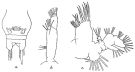
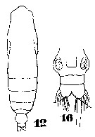
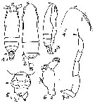
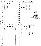
? Eucalanus pileatus-subcrassus : Deevey, 1960 (p.5, Table II, annual abundance) ; | | | | Ref.: | | | Bradford-Grieve, 1994 (p.88, 92, figs.F,M); Al-Yamani & Prusova, 2003 (p.43, figs.F); Conway & al., 2003 (p.168, figs.F,M, Rem.); Goetze, 2003 (p.2322 & suiv.); Mulyadi, 2004 (p.117, figs.F,M, Rem.); Vives & Shmeleva, 2007 (p.882, figs.F,M, Rem.); Goetze & Ohman, 2010 (p.2110, Table 1, 4, A1, Fig.7, molecular study, biogeography); Al Yamani & al., 2011 (p.29, 32, figs.F) | 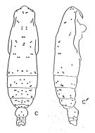 issued from : A. Fleminger in Fishery Bull. natn. Ocean. Atmos. Adm., 1973, 71 (4). [p.987, Fig.11]. As Eucalanus subcrassus. Female: c, habitus (dorsal), c', idem (lateral right side).
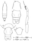
Dorsal and lateral pattern of integumental organs (black point = sites occuring at 100% frequency, o = 80-99% frequency, x = 10-79% frequency, triangle are sites which are also visible in lateral view but which are assigned to dorsal sets);
|
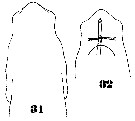
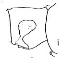 issued from : A. Fleminger in Fishery Bull. natn. Ocean. Atmos. Adm., 1973, 71 (4). [p.968, Fig.1, i (p.969)]. As Eucalanus subcrassus. Female (from 01°16'N, 103°52E): i, genital segment (lateral right side).
|
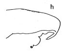 issued from : A. Fleminger in Fishery Bull. natn. Ocean. Atmos. Adm., 1973, 71 (4). [p.968, Fig.1, h (p.969)]. As Eucalanus subcrassus. Female (from 01°16'N, 103°52E)): h, forehead (lateral right side).
|
 issued from : J.G. Greenwood in Proc. R. Soc. Qd, 1976, 87. [p.17, Fig.6]. As Eucalanus subcrassus. Female (from Moreton Bay, E. Australia): a, habitus (dorsal); b, forehead (dorsal); c, urosome (dorsal); d, posterior metasome and urosome (dorsal; another individual); e, endopodal segment 2 of P3. Nota: Genital segment slightly broader than long with maximum width in posterior third; lateral tooth on endopodal segment 2 of P2 to P4 relatively stout. basipodal segment 2 of Mx2 with 5 setae on medial border as found by other authors except Vervoort (1946) who found 4 only. Male: f, P5.
|
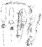
 issued from : R.B.S. Sewell in Mem. Indian Mus., 1929, X. [p.55, Fig.17]. As Eucalanus subcrassus. Female (from N Indian Ocean): a, urosome (ventral); b, Md (mandibular palp); c, Mx1.
|
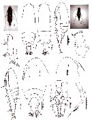
 issued from : F.Y. Al-Yamani & I. Prusova in Common Copepods Northwestern Arabian Gulf : Identification Guide. Kuwait Institute for Scientific Research, 2003. [p.42, Fig.14]. Female: A, habitus (dorsal); B, idem (lateral right side); C, forehead (lateral); D, urosome (dorsal); E, idem (lateral right side); F, Md (mandibular palp). Nota: Prosome nearly 3.4 times as long as wide, 5.7 times urosome.
|
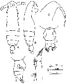
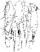
 issued from : T. Mori in The pelagic Copepoda from the neighbouring waters of Japan, 1937 (2nd edit., 1964). [Pl.9, Figs.1-6]. As Eucalanus subcrassus. Female: 1, habitus (dorsal); 4, Md (mandibular palp); 6, Mx1 (without 1st segment of basipodite). male: 2-3, habitus (dorsal and lateral, respectively); 5, left P5.
|
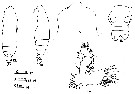 issued from : G.D. Grice in Fish. Bull. Fish and Wildl. Ser., 1962, 61. [p.182, Pl.3, Figs.13-17]. As Eucalanus subcrassus. Female (from equarorial Pacific): 13-14, habitus (dorsal and lateral, respectively); 15, forehead (dorsal); 16, urosome (dorsal); 17, Mx1. Nota: According to Vervoort (1946) there are 4 setae on the 2nd basal segment on Mx1, the present specimen, however, have 5 setae.
|
 Issued from : W. Giesbrecht in Systematik und Faunistik der Pelagischen Copepoden des Golfes von Neapel und der angrenzenden Meeres-Abschnitte. Fauna Flora Golf. Neapel, 1892, 19 , Atlas von 54 Tafeln. [Taf. 35, Figs.12, 16]. As Eucalanus subcrassus. Female: 12, habitus (dorsal); 16, urosome (ventral).
|
 Issued from : W. Giesbrecht in Systematik und Faunistik der Pelagischen Copepoden des Golfes von Neapel und der angrenzenden Meeres-Abschnitte. Fauna Flora Golf. Neapel, 1892, 19 , Atlas von 54 Tafeln. [Taf. 35, Figs.31, 32]. As Eucalanus subcrassus. Female: 31, head (dorsal); 32, forehead (ventral).
|
 issued from : N. Phukham in Species diversity of calanoid copepods in Thai waters, Andaman Sea (Master of Science, Univ. Bangkok). 2008. [p.208, Fig.82]. Female (from W Malay Peninsula): a-b, habitus (dorsal and lateral, respectively); c, urosome (dorsal); d, Md (mandibular palp); e, forehead (lateral); f, Md (gnathobase); g, P2. Male: h-i, habitus (dorsal and lateral, respectively); j, forehead (lateral); k, P5. Body length after drawings: F = 2.50 mm; M = 1.893 mm.
|
 issued from : Mulyadi in Published by Res. Center Biol., Indonesia Inst. Sci. Bogor, 2004. [p.118, Fig.67]. Female (from Indonesian Seas): a-b, habitus (dorsal and lateral, respectively); c, A2; d, Md (palp); e, Md (gnathobase); f, P1; g, P2. Nota: Prosome 5.8 times longer than urosome.Basis of Md with only 3; endopd 1 with 2 inner setae, endopod segment 2 with 4 setae, reaching proximal part of exopod. Male: h, habitus (dorsal); i, rostrum (anterior view); j, P5.
|
 Issued from : M.C. Kos in Field guide for plankton. Zool Institute USSR Acad., Vol. I, 1972. After Brodsky, 1962. As Eucalanus subcrassus. Female: 1, habitus (dorsal); 3, same (lateral); 4, forehead (lateral); 5, urosome (dorsal); 6, Md. Male: 2, habitus (dorsal); 7, P5 (left).
| | | | | Compl. Ref.: | | | Suarez-Morales & Gasca, 1997 (p.1525); Alvarez-Cadena & al., 1998 (tab.1,2,3,4); Hsieh & Chiu, 1998 (tab.2); Suarez-Morales & Gasca, 1998 a (p.109); Hernandez-Trujillo, 1999 (p.284, tab.1); Suarez-Morales & al., 2000 (p.751, tab.1); Lopez-Salgado & al., 2000 (tab.1); Lo & al., 2001 (1139, tab.I); Madhupratap & al., 2001 (p. 1345, vertical distribution vs. O2, figs.4, 5: clusters); Hernandez-Trujillo & Suarez-Morales, 2002 (p.748, tab.1); Uysal & al., 2002 (p.18, tab.1); Hwang & al., 2003 (p.193, tab.2); Hsiao & al., 2004 (p.326, tab.1); Chang & Fang, 2004 (p.456, tab.1); Lan & al., 2004 (p.332, tab.1); Lo & al.*, 2004 (p.218, fig.6); Gallienne & al., 2004 (p.5, tab.3); Kazmi, 2004 (p.229); Yin & al., 2004 (p.3); Lo & al., 2004 (p.89, tab.1); Lavaniegos & Jiménez-Pérez, 2006 (p.157, tab.2, 4, Rem.); Lopez-Ibarra & Palomares-Garcia, 2006 (p.63, Tabl. 1, seasonal abundance vs El-Niño); Zuo & al., 2006 (p.162: tab.1, 3, abundance, fig.8: stations group); Hwang & al., 2006 (p.943, tabl. I); Hwang & al., 2007 (p.24); Dur & al., 2007 (p.197, Table IV); Jitlang & al., 2008 (p.65, Table 1); ? Wishner & al., 2008 (p.163, Table 2, fig.8, oxycline); Lopez Ibarra, 2008 (p.1, Table 1, figs.11, 16: abundance, Table 3: N, C isotopes, figs.17, 18, 19, 20, 22, 24, 25, 26, Annexe 2, Table 4: index trophic); Ayon & al., 2008 (p.238, Table 4: Peruvian samples); Lan Y.C. & al., 2008 (p.61, Table 1, % vs stations); Tseng L.-C. & al., 2008 (p.153, Table 2, fig.5, occurrence vs geographic distribution, indicator species); Tseng & al., 2008 (p.402, Table 2); Tseng L.-C. & al., 2008 (p.46, table 2, abundance vs moonsons, table 3: indicator species); C.-Y. Lee & al., 2009 (p.151, Tab.2); Tseng & al., 2009 (p.327, fig.5, feeding); Zhang W & al., 2009 (p.261, table 2); Hwang & al., 2009 (p.49, fig.4, 5); Cornils & al., 2010 (p.2076, Table 3); Hernandez-Trujillo & al., 2010 (p.913, Table 2); W.-B. Chang & al., 2010 (p.735, Table 2, abundance); Xu & Gao, 2011 (p.514, figs.3, 4, Table 2: optimal salinity); Hsiao S.H. & al., 2011 (p.475, Appendix I); Kâ & Hwang, 2011 (p.155, Table 3: occurrence %); Hsiao & al., 2011 (p.317, Table 2, fig.6, indicator of seasonal change); Tseng L.-C. & al., 2011 (p.239, Table 3, abundance %); Tseng L.-C. & al., 2011 (p.47, Table 2, occurrences vs mesh sizes); Pillai H.U.K. & al., 2011 (p.239, Table 3, vertical distribution); Guo & al., 2011 (p.567, fig.6, table 2, abundance vs spatial distribution, indicator); Lavaniegos & al., 2012 (p. 11, Table 1, seasonal abundance, Appendix); Tseng & al., 2012 (p.621, Table 3: abundance, indicator species); Palomares-Garcia & al., 2013 (p.1009, Table I, fig.7, abundance vs. environmental factors); in CalCOFI regional list (MDO, Nov. 2013; M. Ohman, comm. pers.); Tachibana & al., 2013 (p.545, Table 1, seasonal change 2006-2008); Tseng & al., 2013 (p.507, seasonal abundance); Tseng & al., 2013 a (p.1, Table 3, abundance); Rakhesh & al., 2013 (p.7, Table 1, abundance vs stations); Mendoza Portillo, 2013 (p.37: Fig.7, seasonal dominance, p.42: fig.10, biomass); Oh H-J. & al., 2013 (p.192, Table 1, occurrence); Hwang & al., 2014 (p.43, Appendix A: seasonal abundance); Lopez-Ibarra & al., 2014 (p.453, fig.6, biogeographical affinity) ; Nakajima & al., 2015 (p.19, Table 3: abundance); Zakaria & al., 2016 (p.1, Table 1, Rem.); Jackson & Smith, 2016 (p.305, figs. 3, 4, 5, vertical abundance vs day/night cycle); Marques-Rojas & Zoppi de Roa, 2017 (p.495, Table 1); Hirai & al., 2020 (p.1, Fig. 5: cluster analysis (OTU), spatial distribution). | | | | NZ: | 16 | | |
|
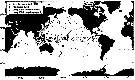
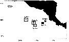
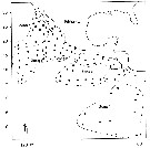
Distribution map of Subeucalanus subcrassus by geographical zones
|
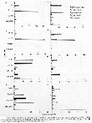
| | | | | | | | | | | |  issued from : C.T. Achuthankutty, N. Ramaiah & G. Padmavati in Pelagic biogeography ICoPB II. Proc. 2nd Intern. Conf. Final report of SCOR/IOC working group 93, 9-14 July 1995. Workshop Report No. 142, Unesco, 1998. [p.8, Fig.6]. issued from : C.T. Achuthankutty, N. Ramaiah & G. Padmavati in Pelagic biogeography ICoPB II. Proc. 2nd Intern. Conf. Final report of SCOR/IOC working group 93, 9-14 July 1995. Workshop Report No. 142, Unesco, 1998. [p.8, Fig.6].
Salinity ranges for E. (= Subeucalanus) subcrassus in coastal and estuarine waters of Goa (India)..
Shaded area indicates the range of higher abundance. |
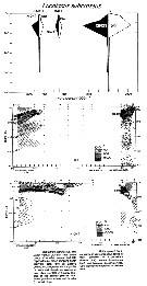
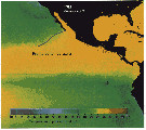
 Issued from : E. Goetze & M.D. Ohman in Deep-Sea Res. II, 2010, 57. [p.2119, Fig.7]. Issued from : E. Goetze & M.D. Ohman in Deep-Sea Res. II, 2010, 57. [p.2119, Fig.7].
Biogeographic distribution of Subeucalanus subcrassus, an equatorial species in the Pacific and Indian Oceans.
Solid circles mark sampling locations of specimens whose species identity was verified by DNA sequencing of 165 rRNA.
Note: The 'positive' records plotted from Lang (1965) are a subset of her original material. |
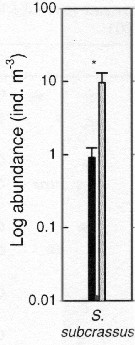 Issued from : S.-H. Hsiao, S. Kâ, T.-H. Fang & J.-S. Hwang inHydrobiologia, 2011, 666. [p.326, Fig.6]. Issued from : S.-H. Hsiao, S. Kâ, T.-H. Fang & J.-S. Hwang inHydrobiologia, 2011, 666. [p.326, Fig.6].
Variations in the most abundant copepod species (mean ± SE) along the transect in the boundary waters between the northern part Taiwan Strait and the East China Sea i March (black bar) and October (grey bar) 2005 (Mann-Whitney U test, sig. *P <0.05.
See drawings of Hydrological conditions and superficial marine currents in Calanus sinicus. |
 Issued from : M.L. Jackson & S.L. Smith in J. Plankton Res., 38 (2). [p.310, Fig.2. Issued from : M.L. Jackson & S.L. Smith in J. Plankton Res., 38 (2). [p.310, Fig.2.
Vertical profiles for Eucalanidae during day night cycles. Numbers of individuals per m3 nare given for each depth interval in the upper 200 m.
(A): Cycle 2-Day; (B) Cycle2-Night; C: Cycle 3-Day; D: Cycle 3-Night; E: Cycle 4-Day, F: Cycle 4-Night; G: Cycle 5-Day, H, Cycleb 5-Night.
Note that depth intervals are not the same in all cycles. See also the site localisations in fig.1 (area of study. zooplankton collected by MOCNESS during summer of 2010. Each cycle at different place in the area of the Costa Rica Dom (Eastern tropical Pacific). |
 Issued from : M.L. Jackson & S.L. Smith in J. Plankton Res., 38 (2). [p.307, Fig.1. Issued from : M.L. Jackson & S.L. Smith in J. Plankton Res., 38 (2). [p.307, Fig.1.
Area of study: Day night cycles were zooplankton were collected with MOCNESS during summer 2010. Cycles 1-5 with day and night tows shown within each cycles. |
 Issued from : M.L. Jackson & S.L. Smith in J. Plankton Res., 38 (2). [p.311, Fig.4. Issued from : M.L. Jackson & S.L. Smith in J. Plankton Res., 38 (2). [p.311, Fig.4.
Median depth of Eucalanidae during day-night cycles.
A: Cycle 2 day and night; B: Cycle 3 day and night; C: Cycle 4 day and night; D: Cycle 5 day and night.
The vertical error bar lines represent the upper and lower median depth range. |
 Issued from : Y.-Q. Chen in CalCOFI Rep., 1986, XXVII. [Fig.3, p.211]. As Eucalanus subcrassus (= Subeucalanus subcrassus): Vertical abundance of females, males and late copepodites. Issued from : Y.-Q. Chen in CalCOFI Rep., 1986, XXVII. [Fig.3, p.211]. As Eucalanus subcrassus (= Subeucalanus subcrassus): Vertical abundance of females, males and late copepodites.
Nota: Samples collected in May-June 1974 with an opening-closing bongo nets (mesh apertures of both nets 0.330 mm and 0.220 mm) from Baja California to Galapagos Is.
Nota: This species was the one of most abundant copepods (12.8% of the total catch in combined day and night samples. The trend of vertical distribution was similar to that of E. subtenuis, occurring mainly above 200 m, but the overall vertical range was deeper. The vertical range of males was shallower than that of females and extended to 250 m in day samples and 150 m in night samples. (see chart Figs.1, 12, 13 in Eucalanus subtenuis). |
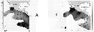 Issued from : G.A. Lopez Ibarra in Tesis, Inst. Politec. Nac., CICIMAR, 2008. [p.48, Fig. 22 and p.51, Fig.24] Issued from : G.A. Lopez Ibarra in Tesis, Inst. Politec. Nac., CICIMAR, 2008. [p.48, Fig. 22 and p.51, Fig.24]
Spatial distribution of the isotopic values from the dominant species for localities (see map for the different zones: a to f). A: δ13C; B: δ15N.
Nota: Sampling in Julio to December 2003, with a Bongo net (333 µm mesh aperture) from obliquely drawing from 200 m depth to surface.
Cf. Map of the 6 zones sampled. |
 Issued from : G.A. Lopez Ibarra in Tesis, Inst. Politec. Nac., CICIMAR, 2008. [p.12, Fig. 1] Issued from : G.A. Lopez Ibarra in Tesis, Inst. Politec. Nac., CICIMAR, 2008. [p.12, Fig. 1]
Eastern tropical Pacific zones sampled: .
Zone a: western coast of mexican Baja California (part of the south California Current).
Zone b: region of the mexican shore.
Zone c: oceanic region off Mexico.
Zone d: central shore region.
Zone e: oceanic central region.
Zone f: oceanic equatorial region. |
 Issued from : G.A. Lopez Ibarra in Tesis, Inst. Politec. Nac., CICIMAR, 2008. [p.27, Fig.9]. Issued from : G.A. Lopez Ibarra in Tesis, Inst. Politec. Nac., CICIMAR, 2008. [p.27, Fig.9].
Superficial temperature in summer 2003 in the eastern tropical Atlantic (°C)
Note the front between the California Current and the North Equatorial Current (blue line on the map). |
 Issued from : G.A. Lopez Ibarra in Tesis, Inst. Politec. Nac., CICIMAR, 2008. [p.37, Table 3] Issued from : G.A. Lopez Ibarra in Tesis, Inst. Politec. Nac., CICIMAR, 2008. [p.37, Table 3]
Summary of abundance and stable isotopics δ15N and δ13C in Subeucalanus subcrassus.
O = omnivore; T = tropical biogeographical affinity; zones (a-f) = Cf. fig.1 in the same author.
Cf. Acartia danae, Centopages furcatus, Eucalanus inermis, Euchaeta indica, E. marina (? = E. rimana), Lucicutia flavicornis, Pleuromamma abdominalis, P. gracilis, P. robusta, Subeucalanus subtenuis, Temora sdiscaudata |
| | | | Loc: | | | South Africa (E & W), Congo, G. of Guinea, Cape Verde Is., off Morocco-Mauritania, Canary Is., Brazil, Barbados Is., Jamaica, Bahia de Mochima (Venezuela), Caribbean Sea, Yucatan, Yucatan (Ascension Bay), E Costa Rica, Cuba, Sargasso Sea, off Bermuda: Station "S" (32°10'N, 64°30'W), ? Delaware Bay (outside) Medit. (Alboran Sea, SW Basin, W Egyptian coast, Lebanon Basin), Red Sea, Indian, Gulf of Oman, G. of Aden, Arabian Sea, Arabian Gulf, UAE coast, Kuwait, Maldive Is., Madagascar (Nosy Bé), Rodrigues Is. - Seychelles, Mascarene Basin, W India, Saurashtra coast, Bombay, Goa - Gujarat, Sri Lanka, Madras, Lawson's Bay, Mandarmani, Hooghly estuary, Godavari region, Bay of Bengal, Andaman Sea (Barren Island), S Burma, Kurau Riv., W Malay Peninsula (Andaman Sea), Australia (W), Perai River estuary (Penang), Straits of Malacca, Thaïland, Indonesia-Malaysia, Sarawak: Bintulu coast, Java (Jakarta-Seribu Islands, off Tegal, off Surabaya, Tioman Is., Lombok Sea, Flores Sea, SW Celebes, Philippines, Viet-Nam (Cauda Bay), Gulf of Tonkin, Hainan (Sanya Bay), Hong Kong, China Seas (Yellow Sea, East China Sea, South China Sea, Xiamen Harbour, Hainan Is.), Kuroshio Current region, Taiwan Strait, Taiwan (S, E, SW, Kaohsiung Harbor, NW, off Danshuei River, N, Mienhua Canyon, NE), S Korea, Geumo Is., Korea Strait, Japan Sea, Japan (Kuchinoerabu Is., Tokyo Bay, Tanabe Bay), Kuroshio region, off S Shikoku Is., Bikini Is., Bering Sea, Pacif. ( W equatorial), Australia (G. of Carpentaria, Great Barrier, Townsville: inshore waters, Moreton Bay, Shark Bay), New Caledonia, Pacif. (equatorial), California, W Baja California (Bahia Magdalena), Gulf of California, G. of Tehuantepec, W Mexico, off W Guatemala, W Costa Rica, Ecuador, off Galapagos, off Peru | | | | N: | 213 | | | | Lg.: | | | (28) F: 2,65-2,1; M: 2,45-1,8; (29) F: 2,113-1,925; M: 1,708-1,666; (34) F: 2,92-1,84; M: 2,7-1,68; (35) F: 2,16-2,1; M: 2,16-2,08; (47) F: 2,68-2,35; M: 2,4; (91) F: ±2,5; M: ±2,4; (101) F: 2,52-2,24; (125) F: 2,82-2,77; M: 2,52; (150) F: 2,62-2,3; M: 2,02; ? (199) F: 2,81-2,28; M: 2,2; (207) F: 2,77-2,65; M: 2,56-2,36; (290) F: 1,95-2,35; M: 1,9-2,2; (332) F: 2,5-2,44; M: 2,65-1,92; (334) F: 2,1-1,9; M: 1,8-1,7; (530) F: 2,5; M: 2,4; (786) F: 2,81-2,1; (795) F: 2,5; M: 2,4; (937) F: 2,12-2,54; (991) F: 1,93-2,88; M: 2,4; (1122) F: 1,9-1,95; M: 1,64; {F: 1,84-2,92; M: 1,64-2,70} | | | | Rem.: | epipelagic, sometimes mesopelagic. Sargasso Sea: 1500-2000 m.
For Itoh (1970 a, fig.2, from co-ordonates) the Itoh's index value of the mandibular gnathobase = 185.
After Mulyadi (2004, p.118) the close similarity between this species and S. pileatus has led some authors (Deevey, 1960; Lang, 1963; Roe, 1972) to treat the wo as one taxon, and to suggestions that they may be conspecific (Grice, 1962; Bjornberg, 1963). Grice (1962) noted the differences between females of the two species, and a detailed description of S. pileatus by Vervoort (1946) stated that there are 4 setae on the basis of mandible.
See in DVP Conway & al., 2003 (version 1) | | | Last update : 05/10/2021 | |
|
|
 Any use of this site for a publication will be mentioned with the following reference : Any use of this site for a publication will be mentioned with the following reference :
Razouls C., Desreumaux N., Kouwenberg J. and de Bovée F., 2005-2025. - Biodiversity of Marine Planktonic Copepods (morphology, geographical distribution and biological data). Sorbonne University, CNRS. Available at http://copepodes.obs-banyuls.fr/en [Accessed January 05, 2026] © copyright 2005-2025 Sorbonne University, CNRS
|
|
|
|


;)
;)
;)
;)
;)
;)
;)
;)
;)
;)
;)
;)
;)

;)
;)
;)
;)
;)
;)
;)
;)