|
|
 |
Fiche d'espèce de Copépode |
|
|
Calanoida ( Ordre ) |
|
|
|
Calanoidea ( Superfamille ) |
|
|
|
Paracalanidae ( Famille ) |
|
|
|
Paracalanus ( Genre ) |
|
|
| |
Paracalanus parvus (Claus, 1863) (F,M) | |
| | | | | | | Syn.: | Calanus parvus Claus, 1863 (p.173, figs.F,M);
Paracalanus parvus : Giesbrecht, 1892 (p.164); no T. Scott, 1894 b (p.26); no Sewell, 1929 (p.68, figs.F,M); ? 1947 (p.51); no Mori, 1929 (p.171, Figs.F,M); 1937 (1964) (p.29, figs.F,M); ? Tanaka, 1956 c (p.369, Rem.F,M);
? Paracalanus parvus Boeck,1864;
Paracalanus parvus borealis Wolfenden, 1905 (1906) (p.997);
Paracalanus parvus perplexus Norman & Scott, 1906;
Piezocalanus lagunaris Grandori, 1912 (p.98, figs.F,M); Carazzi & Grandori, 1912 (p.9, 38); Pesta, 1920 (p.504);
? Paracalanus mariae (M) Brady, 1918 (p.17, figs.M);
Scolecithrix ancorum Oliveira, 1947;
? Paracalanus intermedius Shen & Bai, 1956 (p.219, figs.F,M);
no Paracalanus parvus : Dakin & Colefax, 1940 (p.93, figs.F,M); Bradford, 1972 (p.34, figs.F,M);
? Calocalanus parvus : Hopcroft & al., 1998 (tab.2, lapsus calami);
? Paracalanus parvus s.l. : Chihara & Murano, 1997 (p.844, Pl.135: F,M);
Paracalanus sp. ( = ? quasimodo) : Uye & Shibuno, 1992 (p.343, Uye & Kaname, 1994 (p.43, length vs. fecal pellet volume);
Paracalanus parvus s.l. : Brinton & al., 1986 (p.228, Table 1); Rezai & al., 2004 (p.486, tab.2, 3, abundance); Beltrao & al., 2011 (p.47, Table 1, 2, 3, fig.3, density vs time); Moon & al., 2012 (p.1, Table 1, 2, figs.10, 11, seasonal & spatial variations); Youn & al., 2012 (p.33, seasonal composition, growth rate); Lee J. & al., 2012 (p.95, Table 2: abundance, annual & seasonal distribution); Seo & al., 2013 (p.448, Table 1, occurrence); Park E.-O. & al., 2013 (p.165, Fig.5, distribution vs stations); Suzuki, K.W. & al., 2013 (p.15, Table 2, 3, 4, estuaries, annual occurrence); Oh H-J. & al., 2013 (p.192, Table 1, occurrence); Ohtsuka & Nishida, 2017 (p.565, 578, Table 22.1, Fig. 22.3).
Paracalanus sp. [s.l.] : Ambler, 1986 a (p.957, ingestion rate vs food concentration: nauplius-copepodids-adults);
? Paracalanus parvus f.minor & major : Hirota & Hara, 1975 (p.115, fig.5);
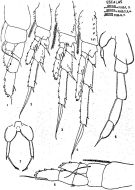
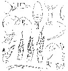
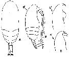
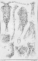
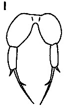
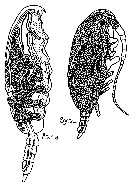
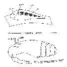
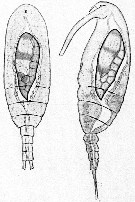
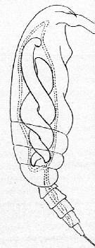
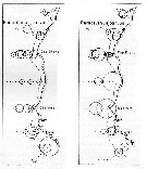
?Paracalanus sp. : Liang & Uye, 1996 (p.219, Rem. : Cf. P. quasimodo). | | | | Ref.: | | | Bourne, 1889 (p.145, figs.figs.F,M); Canu, 1892 (p.169, figs.F,M); Giesbrecht, 1892 (part. p.173, figs.F,M); Sars, 1901 a (1903) (p.17, figs.F,M); Thompson & Scott, 1903 (p.233, 243); Esterly, 1905 (p.140, figs.F,M); Wolfenden, 1905 (1906) (p.997, Rem.); Farran, 1908 b (p.22); ? A. Scott, 1909 (p.27, Rem.); ? Sewell, 1912 (p.353, 358); ? 1914 a (p.208); With, 1915 (p.54, figs.F,M, juv.); Pesta, 1920 (p.500); Lysholm & Nordgaard, 1921 (p.10); Esterly, 1924 (p.86, figs.F,M); Früchtl, 1924 b (p.35); Sars, 1925 (p.24); Rose, 1925 (p.151); Farran, 1926 (p.233); Candeias, 1926 (1929) (p.29, figs.F); Gurney, 1927 (part.?, p.143, figs.F,M, Rem.); Farran, 1929 (p.208, 221); Campbell, 1929 (p.309, Rem.F,M); Rose, 1929 (p.15); Sewell, 1929 (p.38, Rem.); Wilson, 1932 a (p.38, figs.F,M); Rose, 1933 a (p.73, figs.F,M); Jespersen, 1934 (p.49); Farran, 1936 a (p.80); Jespersen, 1940 (p.13); Lysholm & al., 1945 (p.10); Oliveira, 1946 (p.459); Vervoort, 1946 (p.130, Rem.); Sewell, 1948 (part., p.476, Rem: f. indicus & borealis); Davis, 1949 (p.18, Rem.F,M); Brodsky, 1950 (1967) (p.108, figs.F,M); Sewell, 1951 (p.362, 389, Rem.); Farran & Vervoort, 1951 c (n°35, p.3, figs.F,M); Carvalho, 1952 a (p.143, figs.M); Chiba & al., 1957 (p.306); 1957 a (p.11); ? Vervoort, 1957 (p.36, Rem.); Marques, 1959 (p.208, fig.F); Tanaka, 1960 (p.27, Rem.); ? Grice, 1962 (p.183); Vervoort, 1963 b (p.112, Rem.); Shen & Lee, 1963 (p.571, fig.M): Paiva, 1963 (p.24, figs.F,M, anomalies F); Tanaka, 1964 (p.6); Unterüberbacher, 1964 (p.17); Vilela, 1965 (p.5, figs.F,M); Gonzalez & Bowman, 1965 (p.245); Chen & Zhang, 1965 (p.40, 124, figs.F,M); Ramirez, 1966 (p.9, figs.F,M); Marques, 1966 (p.2); Deevey, 1966 (p.161); Saraswathy, 1966 (1967) (p.76); Mazza, 1967 (p.366); Park, 1968 (p.540); Vilela, 1968 (p.11, fig.F: anomalie); Vidal, 1968 (p.22, figs.F,M); Ramirez, 1969 (p.51); Corral Estrada, 1970 (part., p.84, figs.F,M, non Pl.13, fig.5, Rem.: forma "minor" and "major"); Itoh, 1970 (tab.1); Bowman, 1971 b (p.28, figs.F,M, Rem.); Shih & al., 1971 (p.43, 149, 205); Bradford, 1972 (p.34, figs.F,M); Razouls, 1972 (p.94, Annexe: p.15, figs.F); Marques, 1974 (p.13); ? Arcos, 1975 (p.12, figs.F,M); Greenwood, 1976 (p.23); Andronov, 1977 (p.155, fig.F); Bradford, 1978 (p.134: Rem.); Dawson & Knatz, 1980 (p.4, figs.F,M, Rem.); Björnberg & al., 1981 (p.622, fig.F,M); Gardner & Szabo, 1982 (p.168, figs.F,M); Schnack, 1982 (p.89, figs.Mx2, Md, Mxp); Brodsky & al., 1983 (p.214, figs.F,M); Campaner, 1985 (p.10); Ianora & al., 1987 (p.29, figs.F,M, Rem.: Intersexuality); Hiromi, 1987 (p.147, 153, 155, figs.F, Rem.); Nishida, 1989 (p173, figs.1, 2, 3, 5, 6, 7, Table 1, 2, 3: dorsal hump, ultrastructure); Mazzocchi & al., 1995 (p.111, figs.F,M, Rem.); Kim & al., 1993 (p.269); Kang, 1996 (p.409, figs.F, Rem.); Bradford-Grieve & al., 1999 (p.878, 910, figs.F,M); Conway & al., 2003 (p.161, figs.F,M, Rem.); G. Harding, 2004 (p.38, figs.F,M); Boxshall & Halsey, 2004 (p.152, figs.F); Giesecke & Gonzalez, 2004 (p.607, fig.Md); Conway, 2006 (p.12: copepodite stages 1-6, Rem.); Avancini & al., 2006 (p.66, Pl. 35, figs.F,M, Rem.); Vives & Shmeleva, 2007 (p.971, figs.F,M, Rem.); Jagadeesan & al., 2009 (p.239, molecular identification); Kesarkar & Anil, 2010 (Rem.: p.405, fig.F); Blanco-Bercial & al., 2011 (p.103, Table 1, Biol. mol, phylogeny); Laakmann & al., 2013 (p.862, figs.1, 2, 3, 4, 5, Table 1, 2, 3, mol. Biol.); Cornils & Held, 2014 (p.1, cryptic & pseudocryptic forms) | 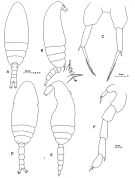 Issued from: M.G. Mazzocchi, G. Zagami, A. Ianora, L. Guglielmo & J. Hure in Atlas of Marine Zooplankton Straits of Magellan. Copepods. L. Guglielmo & A. Ianora (Eds.), 1995. [p.113, Fig.3.17.1]. Female: A, habitus (dorsal); B, idem (lateral right side); C, P5. Nota: Proportional lengths of urosomites and furca 27:17:14:24:18 = 100. A1 not reaching caudal rami, with slightly thickened base. Male: D, habitus (dorsal); E, idem (lateral left side); F, P5. Nota: Proportional lengths of urosomites and furca 9:25:19:17:16:14 = 100. Distal segment of left P5 bearing a longitudinal row of fine hairs. basipod of P2-P4 with very variable ornamentation (spines, spinules and hairs).
|
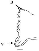 issued from : Giesecke & Gonzalez in Rev. Chil. Hist. Nat., 2004, 77. [p.610, Fig. 2 B]. Schematic drawing of the cutting edge of the lright mandible blade of Paracalanus parvus from Mejillones Bay, Chile . Mean (SD: standard deviation in parenthesis) Itoh's edge index: 254 (29), n = 15 specimens. V1 denote the location of the ventral-most tooth. Scale bar = 0.010 mm. The low edge indice (\"Type I\") suggest that this species is predominantly herbivorous, characterized by a relative thick and flat mandible. This mandibular structure is used to crush diatom frustules, the principal diet.The species might have evolved this type of strategy due to the large thick blunt ventralmost tooth, which could be used to fracture the diatoms (V1 arrow in figure). Once a part of the diatom frustule is cracked, it should be easy to continue breaking it with the help of the nine tiny bicuspid teeth. The large size mandible relative to the body size (width as % of the cephalothorax length = 9.5) indicates that this species is capable of handling larger sized particles, allowing it to feed upon a large size spectrum of diatoms. The shape of mandibles differs slightly from observations made by Schnack (1982) in Kiel Bay (Germany). These morphological differences are due to different feeding modes or food (type and size) availability between Kiel Bay and mejillones Bay.
|
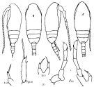
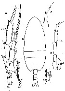
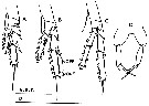
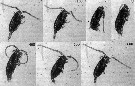
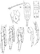 issued from : F.C. Ramirez in Bol. Inst. Biol. Mar., Mar del Plata, 1966, 11. [Lam.IV, Figs.13-19]. Female (from off Mar del Plata): 13, P5; 15, urosome; 16. Male:14, habitus (dorsal); 16, P4; 17, P3; 18, P5; 19, P2.
|
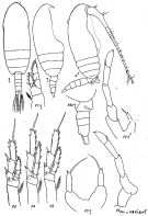
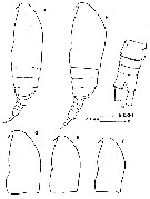
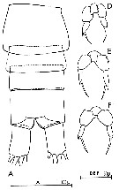
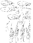
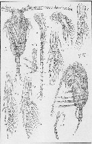
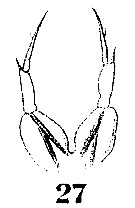
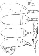 issued from : J. Corral Estrada in Tesis Doct., Univ. Madrid, A-129, Sec. Biologicas, 1970. [Lam.13, figs.1-5]. Female (from Canarias Is.): 3, habitus (dorsal); 4, idem (lateral left side); 5, P4 (see remarks below). Male: 1, habitus (lateral left side); 2, idem (dorsal).
|
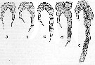
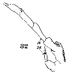
 issued from : J. Corral Estrada in Tesis Doct., Univ. Madrid, A-129, Sec. Biologicas, 1970. [Lam.14]. Male: 1, P1; 2, P2; 3, P3; 4, P4; 5, P5. Female: 6, P1; 7, P5. Size of females forma \"minor\" : 0.74-0.82; females forma \"major\" : 0.92-0.98.
|
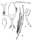
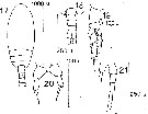
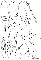
 Issued from : K.A. Brodskii in Calanoida of the Far Eastern Seas and Polar Basin of the USSR. Opred. Fauna SSSR, 1950, 35 (Israel Program for Scientific Translations, Jerusalem, 1967) [p.109, Fig.33°. Female (from N Pacif.): habitus (dorsal and lateral left side); S4E, distal exopodal segment of P4; S5, P5. Male: habitus (dorsal and lateral right side); S5, P5.
|
 issued from : K.A. Brodsky, N.V. Vyshkvartzeva, M.S. Kos & E.L. Markhaseva in Opred Fauna SSSR, 1983, 135. [p.215, Fig.100]. Female & Male (from Japan Sea.).
|
 issued from : C.-j. Shen & S.-o Bai in Acta Zool. sin., 1956, 8 (2). [Pl.II, Figs.7-11]. Female (from Chefoo Harbour): 7, urosome (dorsal); 8, P5. Male: 9, habitus (dorsal); 10, P4; 11, P5.
|
 issued from : A. Ianora, M.G. Mazzocchi & B. Scotto di Carlo in Dis. aquat. Org., 1987, 3 (1). [p.33, Fig.5]. Intersex with fully developed female genital segment and modified male-type (effect of parasitic dinoflagellates into the coelomic cavity/or gut of their host in stage adult).
|
 issued from : A. Ianora, M.G. Mazzocchi & B. Scotto di Carlo in Dis. aquat. Org., 1987, 3 (1). [p.33, Fig.4]. Graded series of modifications in P5 of adult females. From left to right : a, normal. Females possessing an additional 1 (b), 2 (c), and 3 (d) segments in the left ramus approximating that of normal adult males (e).
|
 issued from : J. Hiromi in Bull. Coll. Agr. & Vet. Med., Nihon Univ., 1987, 44. [p.156, Fig.3]. Comparison of diagnostic morphology of P. parvus with that of P. \"parvus\" female. a: P. parvus from Gulf of Maine (lateral view); b-f: P. \"parvus\" from some localities of Japanese waters. b, habitus (lateral); c, urosome (same specimen as b, dorsal), genital segment with cluster of spinules on either side; d-f , head (lateral).
|
 issued from : G.C. Bourne in J. Mar. biol. Ass. U.K., 1889, n. ser. 1.[Pl.XI, Figs.1-3]; Male (from Plymouth): 1, P3; 2, P5; 3, Mxp.
|
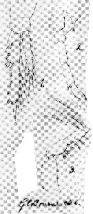
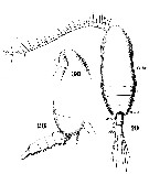
 issued from : C.O. Esterly in Univ. Calif. Publs Zool., 1924, 26 (5). [p.87, Fig. B.). Female (from San Francisco By): 1, posterior margin of thorax and urosome (lateral), showing P5; 2, forehead (lateral); 3, idem (ventral); 4, habitus (dorsal); 10, P2; 12, P4; 15, P5. Male: 5, posterior part of thirax and urosome (ventral); 6, forehead (lateral); 7, anterior portion of head and basal segments of A1 (lateral, right side); 8, posterior border of thorax and P5, 1st and 2nd segments of abdomen (lateral, left side); 9, P1; 11, P2; 13, forehead (ventral); 14, A1; 16, P5.
|
 issued from : C.O. Esterly in Univ. Calif. Publs Zool., 1905, 2 (4). [p.140, Fig.12]. Female (from San Doiego Region): a, P4 (Re3 = 3rd exopodite segment); b, habitus (dorsal); c, P5; d, 2nd endopodite segment of P2. Male: e, P5 (Ps = left leg; Pd = right leg).
|
 issued from : J.M. Bradford in Mem. N. Z. Oceonogr. Inst., 1972, 54. [p.35, Fig.5 (9-12]. Female (from Kaikoura, New Zealand): 10, habitus (dorsal); 11, P5. Male: 9, habitus (dorsal); 12, P5. Scale bars: 1 mm (9, 10); 0.1 mm (12); 0.01 mm (11).
|
 issued from : C. Razouls in Th. Doc. Etat Fac. Sc. Paris VI, 1972, Annexe. [Fig.26, A, D-F]. Female (from Banyuls, G. of Lion); D-F, P5 (from different specimens).
|
 issued from : D.F.R. Arcos in Gayana, Zool., 1975, 32. [Lam.III, Figs.17-21]. With doubt. Female (from Bahia de Concepcion, Chile): 17, habitus (dorsal); 18, urosome (dorsal); 19, P2; 20, P5. Male: 21, P5.
|
 issued from : Y.-S. Kang in J. Korean Fish. Soc., 1996, 29 (3). [p.411, Fig.2]. Female (from Korean waters): A, habitus (dorsal); B, idem (lateral; B': lateral view of anterior portion of the head). Comparison af anterior portion of the head in Paracalanus indicus.
|
 issued from : Y.-S. Kang in J. Korean Fish. Soc., 1996, 29 (3). [p.411, Fig.3]. Female: A-C, P2 to P4; D, P5. OPE: outer proximal edge; ODE: outer distal edge Scale bars 0.2 mm
|
 issued from : Y.-S. Kang in J. Korean Fish. Soc., 1996, 29 (3). [p.412, Table 1]. Morphological comparison of Paracalanus parvus, P. indicus and P. quasimodo based on the scheme of Bradford (1978).
|
 issued from : T.E. Bowman in Smithson. Contr. Zool., 1971, 96. [p.29, Fig.23, b-p]. Female (from Gulf of Maine): b-c, habitus (lateral and dorsal, respectively); d, anal segment and caudal rami (dorsal); e, distal segments of A1; f-h, P2 to P4; i, P5; j, spermathecae from different specimens. Female (from Helgoland): n, habitus (lateral); o, spermathecae from different specimens; p, P3. Nota: Prosome about 3.3-3.4 times as long as urosome, without dorsal hump. Forehead distinctly vaulted. A1 reaching to midlength of caudal ramus. Genital segment without spinules. Surface armature of legs rather sparse, absent from 1st basal segment. Male: k, habitus (lateral); l, left P5 (lateral); m, P5. Nota: Distinguished from the other two western Atlantic males in the '' Parvus group'' by the absence of spinules on the basal segments of the legs.
|
 issued from : G.O. Sars in An Account of the Crustacea of Norway. Vol. IV. Copepoda Calanoida. Published by the Bergen Museum, 1903. [Pl. VIII]. Female. R = rostrum (frontal view); M = Md; m = Mx1; mp2 = Mxp.
|
 issued from : G.O. Sars in An Account of the Crustacea of Norway. Vol. IV. Copepoda Calanoida. Published by the Bergen Museum, 1903. [Pl. IX]. Female & Male.
|
 issued from : K.A. Brodsky, N. V. Vyshkvartzeva, M.S. Kos & E.L. Markhaseva in Opred. Faune SSSR, 1983, 135 (1). [p.215, Fig.100]. Female & Male. P5 female from Brodsky (1950); other figures from the Japan Sea
|
 issued from : K.S. Kesarkar & A.C. Anil in J. mar. Biol. Ass. UK, 2010, 90 (2); [p.405, Table 2]. Characteristics of females.
|
 issued from : K.S. Kesarkar & A.C. Anil in J. mar. Biol. Ass. UK, 2010, 90 (2); [p.407, Fig.5, I]. Female: I, P5.
|
 Issued from : W. Giesbrecht in Systematik und Faunistik der Pelagischen Copepoden des Golfes von Neapel und der angrenzenden Meeres-Abschnitte. Fauna Flora Golf. Neapel, 1892, 19 , Atlas von 54 Tafeln. [Taf.6, Figs.28, 29, 30]. Female: 28, thoracic segment 4+5 and urosome (lateral); 29, habitus (dorsal); 30, forehead (lateral).
|
 Issued from : W. Giesbrecht in Systematik und Faunistik der Pelagischen Copepoden des Golfes von Neapel und der angrenzenden Meeres-Abschnitte. Fauna Flora Golf. Neapel, 1892, 19 , Atlas von 54 Tafeln. [Taf.9, Fig.27]. Female: 27, P5.
|
 Issued from : W. Giesbrecht in Systematik und Faunistik der Pelagischen Copepoden des Golfes von Neapel und der angrenzenden Meeres-Abschnitte. Fauna Flora Golf. Neapel, 1892, 19 , Atlas von 54 Tafeln. [Taf.9, Fig.32]. Male: 32, P5 (posterior view).
|
 Issued from : W. Giesbrecht in Systematik und Faunistik der Pelagischen Copepoden des Golfes von Neapel und der angrenzenden Meeres-Abschnitte. Fauna Flora Golf. Neapel, 1892, 19 , Atlas von 54 Tafeln. [Taf.9, Fig.17]. Female: 17, A1 (ventral view).
|
 Issued from : W. Giesbrecht in Systematik und Faunistik der Pelagischen Copepoden des Golfes von Neapel und der angrenzenden Meeres-Abschnitte. Fauna Flora Golf. Neapel, 1892, 19 , Atlas von 54 Tafeln. [Taf.9, Fig.5]. Male: 5, A1 (ventral view).
|
 issued from : R. Gaudy in Rev. Trav. St. Mar. End., Bull. 27 (42). [p.127, Tableau 4]. Identification of copepodids stages Paracalanus parvus. A: Stage; B: number of swimming legs; C: number of thoracic segments; D: number of abdominal segments; P. 5: 5th thoracic leg.
|
 issued from : G. Trégouboff & M. Rose in Manuel de planctonologie méditerranéenne, 1957, CNRS, Paris. [Pl. 125]. Paracalanus parvus (from NW Mediterranean Sea) parasited by the coelozoic parasit Atelodinium parasiticum (At.pa) in the host's coelome, and in the same individual the parasit Syndinium turbo (Sy.tu).
|
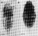 issued from : A. Ianora, B. Scotto di Carlo, M.G. Mazzocchi & P. Mascellaro in J. Plankton Res., 1990, 12 (2). [p.251, Fig.1, A-B]. Healthy adult female specimen of Paracalanus parvus (A). Female parasitized by Syndinium sp. (B). From Gulf of Naples (Italy).
|
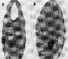 issued from : A. Ianora, B. Scotto di Carlo, M.G. Mazzocchi & P. Mascellaro in J. Plankton Res., 1990, 12 (2). [p.252, Fig.2, A-B]. Longitudinal section of (A) a healthy Paracalanus parvus female (from Gulf of Naples), filled with oocytes (oc) in various phases of development and (B) female infested with Syndinium plasmodial cells (pc) which have destroyed most of the body tissue and lead to sexual castration of the host.
|
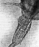
 Issued from : S. Nishida in Mar. Biol., 1989, 101. [p.174, fig.1 and p.175, fig.2]; Paracalanus parvus male (from Sagami Bay): lateral view of prosome showing cephalic dorsal hump (CDH) and measurements taken. d: distance between anterior margin of prosome and CDH; HL: length of CDH. (upper figure): Cephalic dorsal hump (CDH), anterior side to the left. AnP: anterior porez; ApP: apical pore; DP: dorsal plate; TC: area of thin cuticle. For Nishida (1989, p.183) the presence of CDH may partly answer how do the males of those copepods that have little or no modification of their appendages, capture and fertilize females. CDH may function as a short distance receptor to tdentify a conspecificd mate in the early stage of a copulatory process, thus saving energy for appropriate mating; clasping female and spermatophore transfer could be mediated with little-modified P5. It seems that spermatophore transfer itself can be attained in the absence of a highly prehensile P5. This has been achieved in pelagic cyclopoids in which P5 are much reduced into a minute segment with a few setae; the male clasps female with A1 and attaches spermatophore directly to female genital openings (see Hill & Coker, 1930; Uchima, 1998). The mate-recognition system presumed above may partly explain the proliferation of these copepods.
|
 Issued from : S. Nishida in Mar. Biol., 1989, 101. [p.177, Table 3]; Size and location of the cephalic dorsal hump (CDH) measured in the study. d: distance of CDH from anterior margin of prosome; PL: prosome length; HL: length of CDH (as in figure above. Values are mean ± 95 % C.L.). Noe the differences between different species in the Paracalanidae family.
|
 Issued from : S. Nishida in Mar. Biol., 1989, 101. [p.177, Fig.3]; Paracalanus parvus male: Cephalic dorsal hump, anterior side to the left. AnG: secretory cell of anterior gland; AnP: anterior pore; ApG: secretory cell of apical gland; ApP: apical pore; CC: canal cell of antrior gland; EC1: proximal enveloping cell of receptor; EC2: distal enveloping cell of receptor; En: endocuticule; EpC: epidermal cell; Ex: exocuticule; G: Golgi apparatus; M: mitochondrion; MC: muscle cell; N: nucleus; RC: receptor cell; RER: rough endoplasmic reticulum; SG: secretory granule.
|
 Issued from : V.N. Andronov in Russian Acad. Sci. P.P. Shirshov Inst. Oceanol. Atlantic Branch, Kaliningrad, 2014. [p.73, Fig.19: 12 ]. Paracalanus parvus after Wolfenden, 1906. Male P5 with the bent left leg.
|
 Issued from : E. Chatton in Arch. Zool. Exp. & Gen., 1920, 59, [Pl. IV, 39]. Paracalanus parvus female (from Banyuls), with one individual in the stomach of Blastodinium crassum (Dinoflagellate). t.d.: gut; Bl.c.: Blastodiniums crassum.
|
 Issued from : E. Chatton in Arch. Zool. Exp. & Gen., 1920, 59, [Pl. IV, 41]. Paracalanus parvus female (from Banyuls), with in the general cavity a plasmode of Syndinium turbo (Dinoflagellate), which distends the cephalothorax becoming opaque. t.d.: gut; Syn.t.: Syndinium turbo.
Note that the gut is strongly compressed and the aorta (ao) normal.
|
 Issued from : E. Chatton in Arch. Zool. Exp. & Gen., 1920, 59, [p.123, Fig.24]. Paracalanus parvus from Banyuls parasited by Blastodinium crassum (Dinoflagellate), dorsal and lateral views.
|
 Issued from : E. Chatton in Arch. Zool. Exp. & Gen., 1920, 59, [p.190, Fig.96]. Paracalanus parvus female (from Banyuls) parasited by Blastodinium contortum (Dinoflagellate strongly twisted into copepod's gut, oesophagus omitted. Scissiparity very exceptional.
|
 Issued from : E. Chatton in Arch. Zool. Exp. & Gen., 1920, 59, [p.187, Fig.91]. Paracalanus parvus copepodid II parasited by Blastodinium contortum inside the copepod's gut ant a parasite lonely.
|
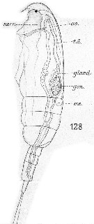 Issued from : E. Chatton in Arch. Zool. Exp. & Gen., 1920, 59, [Pl XII, Fig.128]. Paracalanus parvus copepodid with 3 pedigerous somites showing general structure (lateral view). gon: sketch of genital gonad; t.d.: gut; ; gland.: zymogen region; nerv.: ventral nerve cord; coe: heart; ao: aorta.
|
 Issued from : E. Chatton in Arch. Zool. Exp. & Gen., 1920, 59, [Pl XII, Fig.129]. Paracalanus parvus Copepodid stage V male showing general structure (lateral view). test. testis with its vas deferens (spd.); gr.: oil sac; nerv.: ventral nervous cord; coe.: heart; ao.: aorta; art. rec.: artery issue of bifurcation of the aorta; gl.: zymagen cells of the gut.
|
 Issued from : E. Chatton in Arch. Zool. Exp. & Gen., 1920, 59, [Pl XII, Figs.130, 131]. Paracalanus parvus infested and invaded by the plasmod of Syndinium turbo (Dinoflagellate). 130: young spherical plasmod incapsulated (synd.) against the gut, compressing the gonad (gon.); gland: zymogene region; cae.: heart; t.d.: gut; ao.: aorta. 131: same with an earliset stage of trematod (trem.); caps: capsule of the plasmodd of Syndinium.
|
 Issued from : E. Chatton in Arch. Zool. Exp. & Gen., 1920, 59, [Pl XII, Fig.134i Paracalanus parvus infested and invaded by the plasmod of Syndinium turbo (Dinoflagellate)].
|
 Issued from M. Rose in Résult. Camp. scient. Prince Albert I, 1929, 78, p.16. Remarques concernant Paracalanus parvus identifié lors des campagnes de 1903, 1904, 1906, 1908, 1909, 1910, 1912, 1913 et 1914.
|
 Issued from : A.F. Pasternak & K.O. Kopylov in Oceanology, 1983, 23 (2). åp.241, Fig. 1 & Table 1]. Population density and infestion of P. parvus by Colpoda sp. (Infusorians) in the Black Sea coastal waters.
| | | | | Ref. compl.: | | | Gadeau de Kerville, 1894 (p.81); Cleve, 1904 a (p.194); Pearson, 1906 (p.8, Rem.); Carazzi & Grandori, 1912 (p.7, 38); Chatton, 1920 (p.17, parasite); Wilson, 1932 (p.26); Bogorov, 1939 b (p.707); Massuti Alzamora, 1942 (p.87); Wilson, 1942 a (p.201); Oliveira, 1945 (p.191); Wilson, 1950 (p.275); Fleury, 1950 (p.47, fig.2); Gundersen, 1953 (p.1, 24, Table 21, seasonal abundance); Krishnaswamy, 1953 (p.113); Nakai, 1955 (p.12, chemical composition); Østvedt, 1955 (p.15: Table 3, p.56); Deevey, 1956 (p.216, tab. IV); Grice, 1956 (p.62); Kott, 1957 (p.6, 13); Yamazi, 1958 (p.148, Rem.); Bary, 1959 (p.14, Fig.7, Table 4, correlation T-S): Deevey, 1960 (p.5, Table II, fig.8, 11, annual abundance, Rem.: p.29, fig.18, 19) ; Fagetti, 1962 (p.11); Marshall & Orr, 1962 (tab.1); Ganapati & Shanthakumari, 1962 (p.7, 15); Grice & Hart, 1962 (p.287, table 3,4: abundance); Gaudy, 1962 (p.93, 99, Rem.: p.103, Tableau 4: development); V.N. Greze, 1963 a (tabl.2); Shmeleva, 1963 (p.141); Gaudy, 1963 (p.21, Rem.); Ahlstrom & Thrailkill, 1963 (p.57, Table 5, abundance); Björnberg, 1963 (p.27, Rem.); Northcote & al., 1964 (p.1069,Table 11); Unterüberbacher, 1964 (p.17); De Decker, 1964 (p.16, 24, 30); De Decker & Mombeck, 1964 (p.13); Dimov, 1964 b (p.33, Tableau 1); Anraku & Azeta, 1965 (p.13, Table 2, fish predator); Bodo & al., 1965 (p.219, annual cycle); Martin, 1965 (p.188); Shmeleva, 1965 b (p.1350, lengths-volume -weight relation); Furuhashi, 1966 a (p.295, vertical distribution in Kuroshio region); Neto & Paiva, 1966 (p.21, Table III, annual cycle); Deevey, 1966 (p.155, Table 3, lengths variation), Mazza, 1966 (p.69); Pavlova, 1966 (p.43); Ehrhardt, 1967 (p.737, geographic distribution), Rem.); Matthews, 1967 (p.159, Table 1, Rem.); Fleminger, 1967 a (tabl.1); De Decker, 1968 (p.45); Greze & al., 1968 (p.1066, annual variation); in Oceanology, 1968 p.839, P/B quotient); Séguin, 1968 (p.488); Evans, 1968 (p.14); Berdugo & Kimor, 1968 (p.448); Vinogradov, 1968 (1970) (p.65); Dimov, 1968 (p.506); Delalo, 1968 (p.137); Kovalev, 1968 a (p.441, fig.1); Champalbert, 1969 a (p.626); Kovalev, 1969 a (p.150); Reeve, 1970 (p.894, Rem.: p.904); El-Maghraby & Dowidar, 1970 (p.81); Dowidar & El-Maghraby, 1970 (p.269); Park, 1970 (p.475); Paulmier, 1971 (p.168); Salah, 1971 (p.319); Gamulin, 1971 (p.381, tab.2); Carli, 1971 (p.372, tab.1); Deevey, 1971 (p.224); Timonin, 1971 (p.281, trophic group); Subbaraju & Krishnamurphy, 1972 (p.25, 26 ); Binet, 1972 (p.77); Binet & al., 1972 (p.68, 73); Gaudy, 1972 (p.175, 224, figs. 28-32, annual cycle); Valentin, 1972, p.377: egg diameter = 70 µm); Bainbridge, 1972 (p.61, Appendix Table I: vertical distribution vs day/night, Table II: %, Table IV); Bainbridge & Forsyth, 1972 (p.21, Table I: indictor species); Lefèvre-Lehoërff, 1972 (p.1681); Apostolopoulou, 1972 (p.327, 335); Frolander & al., 1973 (p.277, annual cycles); Arndt & Heidecke, 1973 (p.599, 603, fig.3); Eriksson, 1973 (p.37, fig.10-13, annual cycle); 1973 b (p.113, 117); Desgouille, 1973 (p.1, 131, Rem.: p.136, fig.15); Corral Estrada & Pereiro Muñoz, 1974 (tab.I); Hirota, 1974 (p.1, Table 3, 4, fig.4, 5, 6); Laval, 1974 (p.57, Rem.: p.78, avoidance); Mullin & Evans, 1974 (p.902, efficiency in food chain); Peterson & Miller, 1975 (p.642, 650, Table 3, interannual abundance); Anraku, 1975 (p.79, microdistribution); Patel, 1975 (p.659); Vives & al., 1975 (p.35, tab.II, III, IV); Zismann & al., 1975 (p.59, prey); Porumb, 1976 (p.91); Timonin, 1976 (p.79, vertical distribution); Gaudy, 1976 (p.77, fig.3, Table I, III, production); Grahame, 1976 (p.219, Table X, III); Lakkis & Abboud, 1976 (p.81); Hecq, 1976 (p.443, abundance annual cycle); Peterson & Miller, 1976 (p.14, Table 1, 2, 3, abundance vs interannual variations); Arcos, 1976 (p.85, Rem.: p.91, Table II); Grindley, 1977 (p.341, Table 2); Peterson & Miller, 1977 (p.717, Table 1, seasonal occurrence); Gibson & Grice, 1977 (p.85, Table 1, copper pollution); Timonin & Voronina, 1977 (p.286, fig.5); Ikeda, 1977 c (p.241, Table 1, fig.2, respiration, excretion); Falconetti & Seguin, 1977 (p.188); Carter, 1977 (1978) (p.35); Hanaoka, 1977 (p.267, 300, abundance); Comaschi Scaramuzza, 1978 (p.17); Dessier, 1979 (p.201, 204); Hirota, 1979 a (p.33, Table 2, fig.5); Pipe & Coombs, 1980 (p.223, figs. 1, 2, table 1, vertical distribution); Chen Q-c, 1980 (p.795); Checkley , 1980 (p.430, egg production); 1980 a (p.991, egg production vs. food); Andronov & Maigret, 1980 (p.71, Table 3); Judkins, 1980 (p.475, fig.7: vertical distribution vs O2 minimum); Vaissière & Séguin, 1980 (p.23, tab.1); Hirota 1981 (p.19, Table 1, length-weight-CHN); Gallo, 1981 (p.847); Herman & Mitchell, 1981 (p.739, Table 2, length-volume); Herman & Sameoto, 1981 (p.228, Table 1, 2, abundance); Sreekumaran Nair & al., 1981 (p.493, fig.2 cont.); Bartram, 1981 (p.25, feeding vs development); Arashkevich & al., 1982 (p.477, Table 2, diet); Mackas & Sefton, 1982 (p.1173, Table 1); Castel & Courties, 1982 (p.417, Table II, fig.4, spatial & monthly distribution); Smith S.L., 1982 (p.1331, abundance, monsoon effect); Kovalev & Shmeleva, 1982 (p.82); Vives, 1982 (p.290); Brenning, 1982 (p.2, spatial distribution, T-S diagram, Rem.); Landry, 1983 (p.614, development times vs stages); Huntley & al., 1983 (p.143, Table 2); Turner & Dagg, 1983 (p.11, fig.13, 19, vertical distribution); Price & Paffenhöfer, 1983 (p.116, feeding); Stephen, 1984 (p.161, Distribution vs thermocline & geographic); Pasternak & Kopylov, 1983 (p.240, parasitism); d'Elbée, 1984 (p.25, Fig.6); Tremblay & Anderson, 1984 (p.5); Sameoto, 1984 (p.767, vertical migration); Roe, 1984 (p.356); Kleppel & Pieper, 1984 (p.193, gut contents); Davis C.S., 1984 (p.31, population dynamic, predation); Binet, 1984 (tab.2, 3); Scotto di Carlo & al., 1984 (1043); Guangshan & Honglin, 1984 (p.118, tab.); Gaudy, 1985 (p.279, Tab.3); Binet, 1985 (p.85, tab.3); Brenning, 1985 a (p.23, 24, Table 2); Moraitou-Apostolopoulou, 1985 (p.303, occurrence/abundance in E Mediterranean Sea); Price & Paffenhöfer, 1985 (p.115, feeding); Williams & Collins, 1985 (p.28); Musayeva, 1985 (tab.1); Regner, 1985 (p.11, Rem.: p.24); Mullin & al., 1985 (p.151, Appendix: as ''Paracalanus'', vertical structure v.s. storm & larval fish effects); Jansa, 1985 (p.108, Tabl. I, II, III, IV, V); Garcia-Rodriguez, 1985 a (p.41, 42); Madhupratap & Haridas, 1986 (p.105, tab.1); Brylinski, 1986 (p.457, spatial variations); Yamamoto & Nishizawa, 1986 (p.1729, horizontal distribution); Valentin & al., 1986 (p.117, temporal variations); Hirche, 1989 (p.431, spatial distribution, enzyme activity); Huntley & al., 1986 (p.105, rejected prey); Harris & Malej, 1986 (p.75, Table 5, ammonium excretion); Mikhailovsky, 1986 (p.83, Table 1, ecological modelling); Comaschi Scaramuzza, 1987 (tab.1); Ceccherelli & al., 1987 (p.571, fig.5); Diouf & Diallo, 1987 (p.260); Davis C.S., 1987 (p.947, production); Jimenez-Perez & Lara-Lara, 1988; Tiselius, 1988 (p.215, grazing); Lozano Soldevilla & al., 1988 (p.57); Brylinski & al., 1988 (p.503, size/spatial distribution); Aksnes & Magnesen, 1988 (p.57, population dynamic, production); Hernandez-Trujillo, 1989 a (tab.1); McLaren & al., 1989 (p.560, life history, annual production); Cervantes-Duarte & Hernandez-Trujillo, 1989 (tab.3); Krsinic & Vilicic, 1989 (p.12, tab.3); Mitra & al., 1990 (fig.3); Ohman, 1990 (p.257, fig.); Ianora & al., 1990 (p.249, figs., parsitism effects); Peterson & al., 1990 (p.259, feeding); Tiselius & Jonsson, 1990 (p.23, table 1-4, feeding behaviour); Hirakawa & al., 1990 (tab.3); Krsinic, 1990 (p.337, Table I-III, vertical distribution, comparison bottle-net); Aksnes & Giske, 1990 (p.209, model); Shih & Marhue, 1991 (tab.2, 3); Jouffre & al., 1991 (p.489, lagoon); Hay & al., 1991 (p.1453, Table 2, 5); Hattori, 1991 (tab.1, Appendix); Santos & Ramirez, 1991 (p.79, 80, 82, 83); Nielsen, 1991 (p.1091, egg production); Dai & al., 1991 (tab.1); Gajbhiye & al., 1991 (p.188); Morales C.E. & al., 1991 (p.455, Table I, grazing); Uye, 1991 (p.627, temperature vs length, development); W.T. Peterson & al., 1991 (p.131, egg production, growth rates, secondary production); Hernandez-Trujillo, 1991 (1993) (tab.I); Ayukai & Hattori, 1992 (p.163, Table 5, fecal pellet production rate); Herman, 1992 (p.395, fig.5 b, size distribution by OPC); Huntley & Lopez, 1992 (p.201, Table 1, A1, eggs, egg-adult weight, temperature-dependent production); Bautista & Harris, 1992 (p.41, ingestion rate, gut contents); Norrbin, 1992 (p.6); Guerin-Ancey & David, 1993 (p.119, table 1, biovolume, vertical distribution); Hwang & Choi, 1993 (tab.3); Seguin & al., 1993 (p.23); Tiwari & Nair, 1993 (p.67); Kouwenberg, 1993 (p.215, fig.3, seasonal abundance); 1993 a (p.281, fig.3, 4, sex ratio); Hoffmeyer, 1994 (p.303); Godhantaraman, 1994 (tab.6, 7); Myung & al., 1994 (tab.1); Munk & Nielsen, 1994 (p.1225, fig.4, Table III: egg production, predation); Kouwenberg, 1994 (tab.1); Verheye & al., 1994 (p.155); Palomares Garcia & Vera, 1995 (tab.1); Lefèvre-Lehoërff & al., 1995 (p.269, annual hydroclimatic variations); Hirakawa & al., 1995 (tab.2); Shih & Young, 1995 (p.71); Santos & Ramirez, 1995 (p.133, Tabl. I, fig.2, 3); Gouda & Panigrahy, 1995 (p.206); Krause & al., 1995 (p.81, Fig.22, abundance, Rem.: p.133); Hajderi, 1995 (p.542); Kotani & al., 1996 (tab.2); Jamet & Ferec-Corbel, 1996 (p.17, tab.1); Siokou-Frangou, 1997 (tab.1); Fernandez de Puelles & al., 1996 (p.97, occurrence: p.100); Falkenhaug & al., 1997 (p.449, spatio-temporal pattern); Sharaf & Al-Ghais, 1997 (tab.1); Go & al., 1997 (tab.1); Park & Choi, 1997 (Appendix); Ramaiah & Nair, 1997 (tab.1); Hure & Krsinic, 1998 (p.26, 100); Hsieh & Chiu, 1998 (tab.2); Noda & al., 1998 (p.55, Table 3, occurrence); Mauchline, 1998 (tab.15, 18, 30, 33, 35, 38, 45, 46, 47, 48, 56, 58, 61, 63, 64); Suarez-Morales & Gasca, 1998 a (p.110); Titelmann & Tiselius, 1998 (343, table 1, 2, 3); Verheye & al., 1998 (p.317, Table II); Gomez-Gutiérrez & Peterson, 1999 (p.637, Table I, II, III, VI, figs.4, 5, 6, 7, abundance, egg production); Hernandez-Trujillo, 1999 (p.284, tab.1); Lavaniegos & Gonzalez-Navarro, 1999 (p.239, Appx.1); El-Serehy, 1999 (p.172, Table 1, occurrence); Dolganova & al., 1999 (p.13, tab.1); Harvey & al., 1999 (p.1, 49: Appendix 5, in ballast water vessel); Halvorsen & Tande, 1999 (p.279, tab.2, 3, Rem.: p.282); Bragina, 1999 (p.195); Goldblatt & al., 1999 (p.2619, tabl. 2); Mackas & Tsuda, 1999 (p.335, Table 1); Fernandez-Alamo & al., 2000 (p.1139, Appendix); Razouls & al., 2000 (p.343, Appendix); El-Sherif & Aboul Ezz, 2000 (p.61, Table 3: occurrence); Ueda & al., 2000 (tab.1); Seridji & Hafferssas, 2000 (tab.1); Sautour & al., 2000 (p.531, Table II, abundance); Escribano & Hidalgo, 2000 (p.283, tab.2); Selifonova, 2000 (p.68, tab.1); Moraitou-Apostolopoulou & al., 2000 (tab.I); Plounevez & Champalbert, 2000 (p.175, Table III, IV, V, abundance vs fish, Rem.: p.181); d'Elbée, 2001 (tabl. 1); Dalal & Goswami, 2001 (p.22, fig.2); Fransz & Gonzalez, 2001 (p.255, tab.1); Holmes, 2001 (p.39); Hidalgo & Escribano, 2001 (p.159, tab.2); Pardal & Azeiteiro, 2001 (p.25); El-Serehy & al., 2001 (p.116, tab.1: abundance vs transect in Suez Canal); Mackas & al., 2001 (p.685, Tab. 3, 6, fig.3: interannual changes in species composition); Sameoto & al., 2002 (p.13); Mackas & Galbraith, 2002 (p.725, tab.2a, 2b, fig.6,8); 2002 a (p.423, Table 2); Bressan & Moro, 2002 (tab.2); Zerouali & Melhaoui, 2002 (p.91, Tableau I); Peterson & al., 2002 (p.353); Peterson & al. 2002, (p.381, Table 2, fig.7, interannual abundance); Yamaguchi & al., 2002 (p.1007, tab.1); Wang & al., 2002 (p.348); Hernandez-Trujillo & Suarez-Morales, 2002 (p.748, tab.1); Fernandez de Puelles & al., 2003 (p.123, fig.5); Kovalev, 2003 (p.47); Bode & al., 2003 (p.85, Table 1, abundance); Peterson & Keister, 2003 (p.2499, interannual variability); Keister & Peterson, 2003 (p.341, Table 1, 2, abundance, cluster species vs hydrological events); Zagorodnyaya & al., 2003 (p.52); Vukanic, 2003 (139, tab.1); Vieira & al., 2003 (p.S163, Table 2, abundance); Hsiao & al., 2004 (p.326, tab.1); ? Hsieh & al., 2004 (p.397, tab.1); ? Rezai & al., 2004 (p.489, tab.2, Rem.: largo sensu); ? Lo & al.*, 2004 (p.218, fig.6); ? Lo & al., 2004 (p.468, tab.2); Daly Yahia & al., 2004 (p.366, fig.4, tab.1); ? Lan & al., 2004 (p.332, tab.1, tab.2); Fernandez de Puelles & al., 2004 (p.654, fig.7); Shushkina & al., 2004 (p.524, tab.2); Vargas & Gonzalez, 2004 (p.151); Shimode & Shirayama, 2004 (p.607, tab.1, 2); Wang & Zuo, 2004 (p.1, Table 2, dominance, origin); Vukanic & Vukanic, 2004 (p.9, tab. 2, 3); Kazmi, 2004 (Rem.: p.232); Lo & al., 2004 (p.89, tab.1); Mackas & al., 2004 (p.875, Table 2); Gomes & al., 2004 (p.941, vertical migration vs. stratified waters); Licandro & al., 2005 (p.153); Lakkis & al., 2005 (p.152); Obuid Allah & al., 2005 (p.123, occurrence % vs metal contamination); Choi & al., 2005 (p.710: Tab.III); Ashjian & al., 2005 (p.1380: tab.2); Uriarte & Villate, 2005 (p.863, tab.I); Berasategui & al., 2005 (p.485, tab.1); Mackas & al., 2005 (p.1011, 1021, tab.2); Prusova & Smith, 2005 (p.75); Manning & Bucklin, 2005 (p.233, Table 1); Waggett, 2005 (p.17, Table 3.3, behaviour); Rezai & al., 2005 (p.157, Table 2, 5: spatial & temporal variations); Sterza & Fernades, 2006 (p.95, Table 1, occurrence); Berasategui & al., 2006 (p.485: fig.2); Zuo & al., 2006 (p.159, tab.1, abundance, fig.8: stations group); Camatti & al., 2006 (p.46, fig.5); Isari & al., 2006 (p.241, tab.II); Marques & al., 2006 (p.297, tab.III); Lopez-Ibarra & Palomares-Garcia, 2006 (p.63, Tabl. 1, seasonal abundance vs El-Niño, Rem.: p.69, 72, 74); Mageed, 2006 (p.171, Table 4); Knotz & al., 2006 (p.406, enzymology); Hwang & al., 2006 (p.943, tabl. I) ; Dias & Araujo, 2006 (p.63, Rem., chart); Lavaniegos & Jiménez-Pérez, 2006 (p.150, tab.2, 3, Rem.); Mackas & al., 2006 (L22S07, Table 2); Zervoudaki & al., 2006 (p.149, Table I); De Olazabal & al., 2006 (p.966); Varela & al., 2006 (p.272, Table 3, oil spill effects); Escribano, 2006 (p.20, Table 1); Durbin & Casas, 2006 (p.2537, Table 2a, 2b); Hooff & Peterson, 2006 (p.2610); Fernandez de Puelles & al., 2007 (p.338, fig.7); Valdés & al., 2007 (p.103: tab.1); Zakaria & al., 2007 (p.52, Rem.: p.58, Table 1, vs Salinity); Biancalana & al., 2007 (p.83, Tab.2, 3); Busatto, 2007 (p.26, Tab.3); S.C. Marques & al., 2007 (p.213, Table 1, fig.6); Mackas & al., 2007 (p.223, climatic change index); Marques S.C. & al., 2007 (p.725, Table 1, fig.4, climate variability); Zakaria, 2007 (p.238, Table 2, spatial distribution); Castro & al., 2007 (p.486, Table 1, 3, 4, fig.3); Dur & al., 2007 (p.197, Table IV); Krsinic & al., 2007 (p.528); Khelifi-Touhami & al., 2007 (p.327, Table 1); Isinibilir & al., 2008 (p.745: Tab.1); Cabal & al., 2008 (289, Table 1); Ayon & al., 2008 (p.238, Table 4: Peruvian samples); Lan Y.-C. & al., 2008 (p.61, Table 1, % vs stations, Table 2: indicator species); Tseng L.-C. & al., 2008 (p.153, Table 2, fig.5, occurrence vs geographic distribution, indicator species); Tseng L.-C. & al., 2008 (p.46, table 2, abundance vs moonsons, table 3: indicator species, fig.8); Humphrey, 2008 (p.84: Appendix A); Ohtsuka & al., 2008 (Table 4, Rem.: sensu largo species); Morales-Ramirez & Suarez-Morales, 2008 (p.521); Fernandes, 2008 (p.465, Tabl.2); Gaard & al., 2008 (p.59, Table 1, N Mid-Atlantic Ridge); Selifonova & al., 2008 (p.305, Tabl. 2); Shmeleva & al., 2008 (p.31, Table 1); Takahashi & al., 2008 (p.222, Table 2, grazing impact); Gugliandolo & al., 2008 (p.580, bacteria assiociated); Pepin & al., 2008 (p.1, 43, fig.25, interannual variations); Sun X.H. & al., 2008 (p.637, Rem.: population dynamic and egg production); Waggett & Buskey, 2008 (p.111, fig.2, Table 1); Muelbert & al., 2008 (p.1662, Table 1, 3); Rossi, 2008 (p.90: Tableau XII); Pagano, 2009 (p.116); Lopez Ibarra, 2008 (p.1, Table 1: abundance, Table 2: Rem.); C.-Y. Lee & al., 2009 (p.151, Tab.2); Peterson, 2009 (p.73, Rem.: p 78); Galbraith, 2009 (pers. comm.); Chiba & al., 2009 (p.1846, Table 1, occurrence vs temperature change); Skovgaard & Salomonsen, 2009 (p.425, Table 2) ; Brylinski, 2009 (p.253, Tab.1); Zhang W & al., 2009 (p.261, table 2); Labat & al., 2009 (p.1746, Table 2); Licandro & Icardi, 2009 (p.17, Table 4); Telesh & al., 2009 (p.18: Table 2.1); Lan Y.-C. & al., 2009 (p.1, Table 2, % vs hydrogaphic conditions); Calliari & Tiselius, 2009 (p.111); Zervoudaki & al., 2009 (p.1475, fig.2); Primo & al., 2009 (p.341, Table1, interannual variations); C.E. Morales & al., 2010 (p.158, Table 1: ?); Hirst & al., 2010 (p.2193, sex ratio); Viñas & al., 2010 (p.177, body dimensions vs bivolume); Hafferssas & Seridji, 2010 (p.353, Table 2, 3); Eloire & al., 2010 (p.657, Table II, temporal variability); Lidvanov & al., 2010 (p.356, Table 3); Hernandez-Trujillo & al., 2010 (p.913, Table 2); Cornils & al., 2010 (p.2076, Table 3, Fig.5); Schnack-Schiel & al., 2010 (p.2064, Table 2: E Atlantic subtropical/tropical); Mazzocchi & Di Capua, 2010 (p.426); Medellin-Mora & Navas S., 2010 (p.265, Tab. 2); Fazeli & al., 2010 (p.153, Table 1); W.-B. Chang & al., 2010 (p.735, Table 2, 4, fig.5, abundance); Sun & al., 2010 (p.1006, Table 2); Dvoretsky & Dvoretsky, 2010 (p.991, Table 2); Hafferssas & al., 2010 (p.1281, Table III, abundance vs spatial distribution); Isinibilir, 2010 (p.233, abundance %); Hsiao S.H. & al., 2011 (p.475, Appendix I); Maiphae & Sa-ardrit, 2011 (p.641, Table 2, 3, Rem.); Guo & al., 2011 (p.567, fig.6, abundance vs spatial distribution); ); Pepin & al., 2011 (p.273, Table 2, seasonal abundance); El-Sherbiny & al., 2011 (p.837, seasonal abundance), Sun X.-H. & al., 2011 (p.741, figs.5. 3, 4, tab.I, II, production); Di Mauro & al., 2011 (p.69, biovolume); Magris & al., 2011 (p.260, abundance, interannual variability); S.C. Marques & al., 2011 (p.59, Table 1); Chen H; & al., 2011 (p.84, spatial & temporal variations); Zhang G.-T. & Wong, 2011 (p.277, fig.6, 7, 8, abundance, indicator); Hsiao & al., 2011 (p.317, Table 2, 3, fig.6, indicator of seasonal change); Keister & al., 2011 (p.2498, interannual variation); Turner & al., 2011 (p.1066, Table II, abundance 1998-2008); Fileman & al., 2011 (p.403, abundance vs bloom condition); Menéndez & al., 2011 (p.281, tidal effect); Mazzocchi & al., 2011 (p.1163, Table I, II, fig.6, long-term time-series 1984-2006); Isari & al., 2011 (p.51, Table 2, abundance vs distribution); Zervoudaki & al., 2011 (p.45, fig.3, abundance: Turkish Straits); Tseng L.-C. & al., 2011 (p.239, Table 3, abundance %); Jose & al., 2012 (p.20, fig.3 a,b,c: % vs monsoon); Van Ginderdeuren & al., 2012 (p.3, Table 1); Postel, 2012 (p.327, Table 1); Delpy & al., 2012 (p.1921, Table 2); Uysal & Shmeleva, 2012 (p.909, Table I); DiBacco & al., 2012 (p.483, Table S1, ballast water transport); Zizah & al., 2012 (p.79, Tableau I, Rem.: p.86, 89); Lee D.B. & al., 2012 (p.88, co-occurrence, abundance, feeding); Miloslavic & al., 2012 (p.165, Table 2, transect distribution); Salah S. & al., 2012 (p.155, Tableau 1); Vidjak & al., 2012 (p.243, Rem.: p.253); Aubry & al., 2012 (p.125, table 3, fig.1, interannual variation); Johan & al., 2012 (2013) (p.1, Table 1); Guenther & al., 2012 (p.405, 411); Stefanova & al., 2012 (p.403, Table 2, interannual abundance); Tseng & al., 2012 (p.621, Table 3: abundance); Huo & al., 2012 (p.1, Table 1: dominance); Jean & al., 2012 (p.12, Table 3, protein vs environmental metal stress); Johan & al., 2012 (p.647, Table 1, 2, fig.2, salinity range); Bode & al., 2012 (p.108, spatial distribution vs time-series, % biomass); Gonçalves & al., 2012 (p.321, abundance vs climatic variability); Mazzocchi & al., 2012 (p.135, annual abundance 1984-2006); Menéndez & al., 2012 (p.389, Table 1: seasonal abundance); Lavaniegos & al., 2012 (p. 11, Table 1, fig.3, seasonal abundance, Appendix); Spinelli & al., 2012 (p.39, potential prey for fish); Aguirre & al., 2012 (p.341, Table I: abundance vs season); Rekik & al., 2012 (p.336, Table 1, abundance); Takahashi M. & al., 2012 (p.393, Table 2, water type index); Gusmao & al., 2013 (p.279, Table 3, fig.2, sex-specific predation by fish); Gusmao & al., 2013 a (p.300, Rem., sex ratio); Gubanova & al., 2013 (in press, p.4, Table 4, fig.2); Li C. & al., 2013 (p.101, feeding); in CalCOFI regional list (MDO, Nov. 2013; M. Ohman, comm. pers.); Gissi & al., 2013 (p.86, Table 3, copper toxicity); Tachibana & al., 2013 (p.545, Table 1, Rem: s.l., seasonal change 2006-2008); Tseng & al., 2013 (p.507, seasonal abundance); Jang & al., 2013 (p.1035, egg production, growth rate vs. environmental factors); Jagadeesan & al., 2013 (p.27, Table 3, 5, seasonal variation); Anjusha & al., 2013 (p.40, Table 3, abundance & feeding behavior); Sobrinho-Gonçalves & al., 2013 (p.713, Table 2, fig.8, seasonal abundance vs environmental conditions); Zhang H. & al., 2013 (p.57, Rem. p.58); Varadharajan & Soundarapandian, 2013 (p.2: occurrence vs stations); Hirai & al., 2013 (p.1, Table I, molecular marker); Santhanam & al;, 2013 (p.243, egg production vs temperature & algal food); Terbiyik Kurt & Polat, 2013 (p.1163, Table 2, seasonal distribution); Mendoza Portillo, 2013 (p.37: Fig.7, seasonal dominance); El-Serehy & al., 2013 (p.2099, Rem.: p.2101); Lidvanov & al., 2013 (p.290, Table 2, % composition); Batchelder & al., 2013 (p.34, Rem.: p.42); Tiselius & al;, 2013 (p.1657, figs. 3, 5, 6, Table 2, food detection); Fernandez de Puelles & al., 2014 (p.82, Table 1, 3, 6, fig.11, seasonal abundance); Bonecker & a., 2014 (p.445, Table II: frequency, horizontal & vertical distributions); Lopez-Ibarra & al., 2014 (p.453, Table 2, biogeographical affinity) ; Pansera & al., 2014 (p.221, Table 2, abundance); Zaafa & al., 2014 (p.67, Table I, occurrence); Aboul Ezz & al., 2014 (p.283, Rem.: p.284, 287); Zakaria, 2014 (p.3, Table 1, abundance vs 1960-2000); Mazzocchi & al., 2014 (p.64, Table 3, 4, 5, spatial & seasonal composition %); Dias & al., 2015 (p.483, Table 2, abundance, biomass, production, Table 4: % vs. season); Rojas-Herrera & al., 2016 (p.40, Table 2: temporal abundance); Zakaria & al., 2016 (p.1, Table 1, 3, 4); Benedetti & al., 2016 (p.159, Table I, fig.1, functional characters); Ben Ltaief & al., 2017 (p.1, Table III, Summer relative abundance): Jerez-Guerrero & al., 2017 (p.1046, Table 1: temporal occurrence) ; Ohtsuka & Nishida, 2017 (p.565, Fig. 22.3: central station-outermost station in Japanese waters); El Arraj & al., 2017 (p.272, table 1, 2, seasonal composition); Benedetti & al., 2018 (p.1, Fig.2: ecological functional group); Belmonte, 2018 (p.273, Table I: Italian zones); Abo-Taleb & Gharib, 2018 (p.139, Table 5, occurrence %); Chaouadi & Hafferssas, 2018 (p.913, Table II, III, fig.4, 5: occurrence, abundance, seasonal variation); Camatti & al., 2019 (p.1, fig. 6, Table 3, 4, 5); Richirt & al., 2019 (p.3, Table 1, fig.2, 3, 4, 5, abundance changes vs years 1998-2014, table 2: diversity index); Hure M. & al., 2018 (p.1, Table 1: abundance, % composition, Table 2: correlations, Rem.: p.11); Palomares-Garcia & al., 2018 (p.178, fig.3: relative frequency, Table 1); Acha & al., 2020 (p.1, Table 3: occurrence % vs ecoregions, Table 5: indicator ecoregions). | | | | NZ: | 24 | | |
|
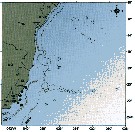
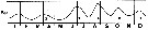
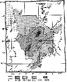
Carte de distribution de Paracalanus parvus par zones géographiques
|
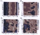
| | | | | | | | | | | | | | | | | |  issued from : A.A. Shmeleva in Bull. Inst. Oceanogr., Monaco, 1965, 65 (n°1351). [Table 6: 7]. Paracalanus parvus (from South Adriatic). issued from : A.A. Shmeleva in Bull. Inst. Oceanogr., Monaco, 1965, 65 (n°1351). [Table 6: 7]. Paracalanus parvus (from South Adriatic).
Dimensions, volume and Weight wet. Means for ca.100 specimens. Volume and weight calculated by geometrical method. Assumed that the specific gravity of the Copepod body is equal to 1, then the volume will correspond to the weight. |
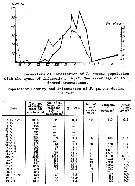
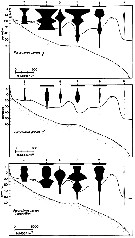
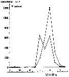
 issued from : P.S.B. Digby in J. Mar. Biol. Ass. U.K., 1950, 29. [p.400, Fig.3]. issued from : P.S.B. Digby in J. Mar. Biol. Ass. U.K., 1950, 29. [p.400, Fig.3].
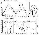
Life history of Paracalanus parvus at station L (5 miles from Plymouth, English Channel).
A: abundance of copepodite stages; B: percentage distribution of stages; C: size-groups of adult females; D: suggested interpretation of generations (or cohorts) succession during the year (1947).
Correlate the size variations with the water temperature at station L4 (p.397, Fig.1).
The author deduces the succession of 6 generations. |
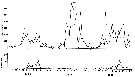
 issued from : P.S.B. Digby in J. Mar. Biol. Ass. U.K., 1950, 29. [p.397, Fig.1]. issued from : P.S.B. Digby in J. Mar. Biol. Ass. U.K., 1950, 29. [p.397, Fig.1].
Temperature of the water at 1 and 30 m depth at station L4 (5 miles from Plymouth, English Channel) during 1947. x: surface readings from closer in-shore. |
 issued from : C. de O. Dias & A.V. Araujo in Atlas Zoopl. reg. central da Zona Econ. exclus. brasileira, S.L. Costa Bonecker (Edit), 2006, Série Livros 21. [p.63]. issued from : C. de O. Dias & A.V. Araujo in Atlas Zoopl. reg. central da Zona Econ. exclus. brasileira, S.L. Costa Bonecker (Edit), 2006, Série Livros 21. [p.63].
Chart of occurrence in Brazilian waters (sampling between 22°-23° S).
Nota: sampling 22 specimens. |
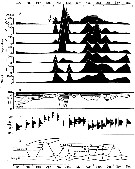
 issued from : J.T. Turner & M.J. Dagg in Biol. Oceanogr., 1983, 3 (1). [p.12, Fig.5]. issued from : J.T. Turner & M.J. Dagg in Biol. Oceanogr., 1983, 3 (1). [p.12, Fig.5].
Vertical and inshore-offshore distributions of paracalanus parvus in relation to the 15°C isotherm at pump stations on the Long Island (NW Atlantic) transect (40°31.8'-39°53.2' N, 72°23.6'-72°59.4' W; October 1978).
Station numbers are given on the top axis, and dark horizontal bars identify stations sampled at night. |
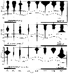 issued from : J.T. Turner & M.J. Dagg in Biol. Oceanogr., 1983, 3 (1). [p.26, Fig.11]. issued from : J.T. Turner & M.J. Dagg in Biol. Oceanogr., 1983, 3 (1). [p.26, Fig.11].
vertical distribution of Paracalanus parvus in relation to positions of the 15°C and 10°C water at the time of sampling during the Long Island NW Atlantic) time series (40°26'N, 72°18'W; October 1978).
Sampling times are given on the bottom axis, and dark horizontal bars identify periods of darkness. |
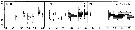
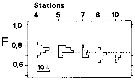 issued from : J.-M; Brylinski, D. Bentley & C. Quishoudt in J. Plankton Res., 1988, 10 (3). [p.507, Fig.5]. Lenth prosome histogramm (in mm) of Paracalanus parvus females (F) in relation with the transect from Boulogne-sur-Mer to Dover, through the Dover Strait (stations 4, 5, 7, 8, 10). issued from : J.-M; Brylinski, D. Bentley & C. Quishoudt in J. Plankton Res., 1988, 10 (3). [p.507, Fig.5]. Lenth prosome histogramm (in mm) of Paracalanus parvus females (F) in relation with the transect from Boulogne-sur-Mer to Dover, through the Dover Strait (stations 4, 5, 7, 8, 10).
Stations 4, 5 off Gris-nez cape, stations 7, 8 and 10 in axis of the Dover Strait..
The dotted line is arbitrary reference. Each stations equidistant. |
 issued from : A. Ianora, B. Scotto di Carlo, M.G. Mazzocchi & P. Mascellaro in J. Plankton Res., 1990, 12 (2). [p.253, Fig.3]. issued from : A. Ianora, B. Scotto di Carlo, M.G. Mazzocchi & P. Mascellaro in J. Plankton Res., 1990, 12 (2). [p.253, Fig.3].
Paracalanus parvus (from Gulf of Naples). Seasonal oscillatio,s in adult (continuous line) and juvenile (dashed line) populations sampled from January 1986 to December 1988 at fixed station (upper graph) and corresponding percentage infection rates for adult females and juveniles parasitized by Syndinium sp. (lower graph).
Specimens infested with Syndinium were markedly seasonal in their occurrence, with highest infection rates coinciding with periods of maximum host abundances. They also showed striking year-to-year fluctuations.
Juveniles were as heavily parasitized as adults, with infection rates of up to 12 % i September 1986. Maximum infection rates for adult females were ± 13 % in September 1988. By contrast, parasitized specimens of the genera Clausocalanus and calocalanus were extremely rare (< 0.1 %).
The dinoflagellate Blastodinium was occasionally observed in females and juveniles. |
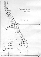
 issued from : U. Brenning in Wiss. Z. Wilhelm-Pieck-Univ. Rostock - 31. Jahrgang 1982. Mat.-nat. wiss. Reihe, 6. [p.1, Figs.1, 2]. issued from : U. Brenning in Wiss. Z. Wilhelm-Pieck-Univ. Rostock - 31. Jahrgang 1982. Mat.-nat. wiss. Reihe, 6. [p.1, Figs.1, 2].
Spatial distribution for ''Paracalanus parvus'' from 8° S - 26° N; 16°- 20° W, for diferent expeditions (V1: Dec. 1972- Jan. 1973 and VI: May 74). |
 issued from : U. Brenning in Wiss. Z. Wilhelm-Pieck-Univ. Rostock - 31. Jahrgang 1982. Mat.-nat. wiss. Reihe, 6. [p.3, Figs.5]. issued from : U. Brenning in Wiss. Z. Wilhelm-Pieck-Univ. Rostock - 31. Jahrgang 1982. Mat.-nat. wiss. Reihe, 6. [p.3, Figs.5].
Spatial distribution for ''Paracalanus parvus'' from 8° S - 26° N; 16°- 20° W, and Namibia (SW-Africa) for diferent expeditions (V1: Dec. 1972- Jan. 1973; VI: May 74; and VIII).
SO: Southern Surface Water (S °/oo: 34,50; T°C: 29,0); ND: Northern Water of the Surface Layer (S °/oo: 37,5; T°C: 21,0); SD: Southern Deep Water of the surface layer (S °/oo: 35,33; T°C: 13,4). See commentary in Temora stylifera and Brenning (1985 a, p.6).
Nota: This species is euryecological form. But the actual systematic status of ''P. parvus'' is still uncertain. |
 issued from : U. Brenning in Wiss. Z. Wilhelm-Pieck-Univ. Rostock - 31. Jahrgang 1982. Mat.-nat. wiss. Reihe, 6. [p.2, Figs.4]. issued from : U. Brenning in Wiss. Z. Wilhelm-Pieck-Univ. Rostock - 31. Jahrgang 1982. Mat.-nat. wiss. Reihe, 6. [p.2, Figs.4].
Spatial distribution for ''Paracalanus parvus'' from Namibia (expedition VIII: 21/9-17/12 1976) |
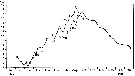
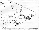
 issued from : R. Gaudy in Tethys, 1972, 4 (1). [p.237, Fig.36]. issued from : R. Gaudy in Tethys, 1972, 4 (1). [p.237, Fig.36].
Schematic quantitative abundance of Paracalanus parvus in the Gulf of Marseille (Mediterranean Sea) established from samples during the period between April 1962 to December 1967.
Gaudy (p.188) points to 5 generations per year.
Nota: Gaudy (p.227) points with certainty 5 generations per year, plus probably 1 generationr epresented by adult forms in November or December. The maximum of adults in August and September. |
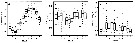
 issued from : S. Eriksson in ZOON, 1976, 4. [p.157, Fig.2]. issued from : S. Eriksson in ZOON, 1976, 4. [p.157, Fig.2].
Seasonal distribution of neritic copepod Paracalanus parvus off Gothenburg (Göteborg), The Skattegatt. (Monthly means for adult specimens during 1968-1973; point : inshore, depth = 10 m; x: offshore, depth > 40 m.
This species has the period of main occurrence during the late part of the summer when the surface water is warmer than 15°C and the whole water mass is warmer than 10°C. The temperature optimum is 10 to 19°C. |
 issued from : S. Eriksson in ZOON, 1976, 4. [p.158, Fig.3, b]. issued from : S. Eriksson in ZOON, 1976, 4. [p.158, Fig.3, b].
Temperature occurrence of neritic copepod Paracalanus parvus off Gothenburg (Göteborg), The Skattegatt.
. Surface salinity of the investigation area varies around 25 p.1000 and the deep water slinity around 34 p.1000. There is a temperature stratification with surface water warmer than 10°C from May to October with maximum of 20°C in August. The coldest period is January to March with surface temperatures of 1-2°C. The deep water ranges between 5 and 10°C.
The hauls were horizontal at 2, 20, and 40 m.
Limits subjectively regarded as the optimum temperature range: 10-19°C. |
 issued from : S. Eriksson in ZOON, 1973, 1. [p.50, Fig.11]. issued from : S. Eriksson in ZOON, 1973, 1. [p.50, Fig.11].
Size distribution of adult females of Paracalanus parvus (offshore station H6:11°30' N, 57°40'.5 E, The Kattegatt) during 1968-70 in the main series. |
 issued from : S. Eriksson in Mar. Biol., 1974, 26. [p.320, Figs. 2-3] issued from : S. Eriksson in Mar. Biol., 1974, 26. [p.320, Figs. 2-3]
Salinity and temperature curves for main series at offshore station H6 (11°30' N, 57°40'.5 E, The Kattegatt) from March 1968 to November 1970. |
 issued from : I.A. McLaren, M.J. Tremblay, C.J. Corkett & J.C. Roff in Can. J. Fish. Aquat. Sci., 1989, 46. [p.573, Fig.11]. issued from : I.A. McLaren, M.J. Tremblay, C.J. Corkett & J.C. Roff in Can. J. Fish. Aquat. Sci., 1989, 46. [p.573, Fig.11].
Annual cycle of Paracalanus parvus on Emerald Bank (43°30'N, 63°00'W), 1979-80.
For convenience, Nov. 1979 sample placed at end after 1980). Upper panel: abundances as proportions of stages (AD: adults). Lower panel: size-frequencies of adult females as proportions.
The samples were obtained by vertical hauls from near bottom (usually 25 m) by Hensen-type nets (one of 0.250 mm mesh and the other of 0.064 mm mesh). |
 issued from : D.M. Checkley Jr. inLimnol. Oceanogr., 1980, 25 (6). [p.994, Fig.2]. issued from : D.M. Checkley Jr. inLimnol. Oceanogr., 1980, 25 (6). [p.994, Fig.2].
Development time of Paracalanus parvus eggs as a function of temperature, determined in the laboratory.
Means and 95% confidence limits of the true means are shown.
A third to a half of eggs did not hatch at 9° and 10°C.
D in days, least-squares regression; D= 432 (T + 2.97) exposant -2.25.
Animais collected in the Sea from Los Angeles during February-March 1975 and August-September 1976.
Nota: The in situ rate of egg production is significantly correlated with chlorophyll a (positive), female length (positive), and temperature (negative). Significant correlations also exist between female length and chlorophyll a (positive) and temperature (negative).
A stepwise multiple linear regression was performed to separate the effects of food, temperature, and female size on the in situ rate of egg production (seestatistical package in Nie & al., 1970).
The conclusion for the author is that variation in the rate of egg production of adult was significantly related to variation in the concentration of chlorophyll a ; variation in female size wqs significantly related to variation in the concentration of chlorophyll a and in temperature; that phytoplankton > 5µ best characterized the food used by P. parvus for the production of eggs; and finally, that an onshore-offshore gradient in food limitation of egg production by P. parvus existed, on average, during 1974-1978 in the sea off southern California. |
 Issued from : M. Anraku in Mar. Biol., 1975, 30. [p.82, Figs. 1, 2]. Issued from : M. Anraku in Mar. Biol., 1975, 30. [p.82, Figs. 1, 2].
Distribution of hydrological factors and abundance of Paracalanus parvus in Oshoro Bay (west Hokkaido, Japan), 30 August 1958, along vertical section from stations 1 to 5 (distance 650 m).
Nota: The plankton samples were collected by means of a plankton pump during the morning hours at the same time as the hydrological observations. Copepodids and adults were counted ans expressed as number of individuals per 20 l.
The distribution of copepods in a limited area seems to be related to the pattern of oceanographic conditions to some extent, but a pattern of contagious distribution is also apparent. See Barnes & Marshall (1951) ; Cassie (1959) ; Boyd (1973). |
 Issued from : M. Anraku in Mar. Biol., 1975, 30. [p.84, Fig.5]. Issued from : M. Anraku in Mar. Biol., 1975, 30. [p.84, Fig.5].
Microdistribution of Paracalanus parvus in Oshoro Bay (west Hokkaido, Japan), 28 August 1958, ascertained by pump along vertical section from station 3.
Nota: After the author, it is clear that the results obtained in the present investigations indicate non-random distribution.
The distribution patterns indicated the presence of inhomogeneous distribution with small swarms and irregular layerings.
Large-scale patchiness of plankton has previously been recorded (see Hardy & Gunther, 1935; Rae & Rees, 1947). The results of the present investigation indicate thet the large-scale patch includes small patches of different sizes in both the horizontal and vertical planes.
Simultaneous measurements of certain physical, chemical, and biological parameters (as the the quantitative and qualitative food particles, the occurrence of predators) are necessary to approach an understanding of copepod microdistribution. |
 Issued from : M. Krause, J.W. Dippner & J. Beil in Prog. Oceanog., 1995, 35. [p.109, Fig.22]. Issued from : M. Krause, J.W. Dippner & J. Beil in Prog. Oceanog., 1995, 35. [p.109, Fig.22].
Horizontal distribution pattern of Paracalanus parvus (individuals per m2) in the winter North Sea.
Collected by WP2-net. Numbers (ind/m3) depth-integrated, extrapoled to the bottom (but at a maximum to a depth of 500 m) and expressed as ind per m2 of water surface. |
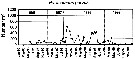
 Issued from : M.-C. Jang, K. Shin, B. Hyun, T. Lee & K.-H. Choi in J. Plankton Res., 2013, 35 (5). [p.1042, Fig.6]. Issued from : M.-C. Jang, K. Shin, B. Hyun, T. Lee & K.-H. Choi in J. Plankton Res., 2013, 35 (5). [p.1042, Fig.6].
Ten-year variation in the monthly distribution of (a) water temperature (°C), (b) salinity, (c) Chl.a (log µg /L and (d) Paracalanus parvus abundance (log10 inds/m3) in Jangmok Bay (34°59'38''N, 128°40'29''E), southern coast of Korea.
Nota: The water temperature in the northern East China Sea region has been increasing steadily since the 1980s at a rate of 0.024°C per year, with the February 18°C isopleths moving nortward. Following yjis sea water temperature rise, mesozooplankton biomass and copepod concentrations have increased in all three seas surrounding the Korean Peninsula, although the reason for this remains unresolved. Seasonal changes in copepod abundance suggest that warming coastel waters are likely to result in increased populations of this species, especially winter populations. |
 Issued from : M.-C. Jang, K. Shin, B. Hyun, T. Lee & K.-H. Choi in J. Plankton Res., 2013, 35 (5). [p.1040, Fig.3, d]. Issued from : M.-C. Jang, K. Shin, B. Hyun, T. Lee & K.-H. Choi in J. Plankton Res., 2013, 35 (5). [p.1040, Fig.3, d].
Weekly/biweekly variations in Paracalanus parvus sex ratio (dark = female; gray = male)from August 2009 to July 2010 in Jangmok Bay.
Nota: The study shows that the sex ratio was highly skewed toward females throughout the year. Ther sex ratio of males to total adults (0.01-0.34) in the present study is a bit higher or closer to the reported range (0.1-0.45, with a mean ratio of 0.2) in adult paracalanids in nature (Kiørboe, 2006). |
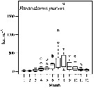
 Issued from : P. Santhanam, N. Jeyaraj & K. Jothiraj in J. Environm. Biol., 2013, 34. [p.245, Tables 1, 2]. Issued from : P. Santhanam, N. Jeyaraj & K. Jothiraj in J. Environm. Biol., 2013, 34. [p.245, Tables 1, 2].
Mean egg production and hatching rate of Paracalanus parvus at different temperatures and in different algal food concentration.
Copepods collected from the Muthupet mangrove waters (10°20'N, 79°35'E). Algal food obtained from aquaculture (Chlorella marina, Dunaliella sp., Isochrysis galbana, Nannochloropsis sp., Coscinodiscus centralis, Chaetoceros affinis, Skeletonema costatum). |
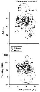 Issued from : K.W. Suzuki, K. Nakayama & M. Tanaka in J. Oceanogr., 2011, 69. [p.25, Fig.7]. Issued from : K.W. Suzuki, K. Nakayama & M. Tanaka in J. Oceanogr., 2011, 69. [p.25, Fig.7].
Bubble plots of densities of the non semi-endemic calanoid Paracalanus parvus sp. in relation to temperature, salinity, and turbidity observed in the Chikugo and Midori River estuaries (south Japan) in 2005 and 2006. |
 Issued from : W.T. Peterson, J.E. Keister & L.R. Feinberg in Prog. Oceanogr., 2002, 54. [p.391, Fig.7]. Issued from : W.T. Peterson, J.E. Keister & L.R. Feinberg in Prog. Oceanogr., 2002, 54. [p.391, Fig.7].
Abundance (number per cubic meter) of Paracalanus parvus at the station NH5 (off Newport, Oregon, at depth 30 m) from May 1996 through September 1999.
Compare with Calanus marshallae and Pseudocalanus mimus at the same station, during El Niño event in 1997-98, the largest of the century. |
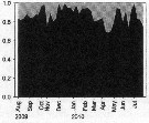
 Issued from : M.G. Mazzocchi, L. Dubroca, C. Garcia-Comas, I. Di Capua & M. Ribera d'Alcalà in Prog. Oceanogr., 2012, 97-100. [p.141, Fig.7]. Issued from : M.G. Mazzocchi, L. Dubroca, C. Garcia-Comas, I. Di Capua & M. Ribera d'Alcalà in Prog. Oceanogr., 2012, 97-100. [p.141, Fig.7].
Average annual cycle of abundance (ind. m3) of Paracalanus parvus at station MC in the period 1984-2006.
iNota: Individual samples collected by vertical tows in the upper 50 m at station MC in the Gulf of Napoli, depth < 100m. |
 Issued from : M.G. Mazzocchi, L. Dubroca, C. Garcia-Comas, I. Di Capua & M. Ribera d'Alcalà in Prog. Oceanogr., 2012, 97-100. [p.139, Fig.3]. Issued from : M.G. Mazzocchi, L. Dubroca, C. Garcia-Comas, I. Di Capua & M. Ribera d'Alcalà in Prog. Oceanogr., 2012, 97-100. [p.139, Fig.3].
Average annual cycle of (a) temperature (*C), (b) salinity (psu), and (c) chlorophyll a concentration (mg m3) integrated in the 0-50 m layer at Station MC (Gulf of Naples) in the period 1984-2006. Box-and-whisker plots have whisker range fixed at 1.5 times the interquartile interval. |
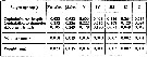
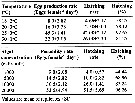
 Issued from : M.D. Viñas, N.R. Diovisalvi & G.D. Cepeda in J. Braz. Oceanogr., 2010, 58 (2). [p.178, Table 1]. Issued from : M.D. Viñas, N.R. Diovisalvi & G.D. Cepeda in J. Braz. Oceanogr., 2010, 58 (2). [p.178, Table 1].
Body dimensions and estimated biovolume of Paracalanus parvus samples on October 18th and November 11th at the permanent coastal station (38°28'S, 57°41'W).
Body wet weight can be derived from measurements of body volume by applying a factor of 1 for specific gravity. Dry weight can be obtained by mulitplyng the wet weight by 0.20 and the carbon content as 40% of the dry weight.
F: female; M: male. |
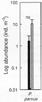 Issued from : S.-H. Hsiao, S. Kâ, T.-H. Fang & J.-S. Hwang inHydrobiologia, 2011, 666. [p.326, Fig.6]. Issued from : S.-H. Hsiao, S. Kâ, T.-H. Fang & J.-S. Hwang inHydrobiologia, 2011, 666. [p.326, Fig.6].
Variations in the most abundant copepod species (mean ± SE) along the transect in the boundary waters between the northern part Taiwan Strait and the East China Sea i March (black bar) and October (grey bar) 2005 (Mann-Whitney U test, sig. ns: P >0.05.
See drawings of Hydrological conditions and superficial marine currents in Calanus sinicus. |
 Issued from : P. Tiselius, E. Saiz & T. Kiørboe in Limnol. Oceanogr., 2013, 58 (5). [p.1659, Table 2]. Issued from : P. Tiselius, E. Saiz & T. Kiørboe in Limnol. Oceanogr., 2013, 58 (5). [p.1659, Table 2].
Duration (milliseconde: ms) of components of feeding behavior of Paracalanus parvus (average ± SD) with Heterocapsa triquetra (Dinoflagellate) as prey.
Filming after coppepods collected in the Gullmar Fjord (west coast of Sweden: Skagerrak).
Nota: In the film cell detection and capture by freely swimming Paracalanus parvus, all behavorial responses were extremely rapid (0.02 - 0.2 s) and involved several mouth appendages. |
 Issued from : P. Tiselius, E. Saiz & T. Kiørboe in Limnol. Oceanogr., 2013, 58 (5). [p.1661, Fig.3]. Issued from : P. Tiselius, E. Saiz & T. Kiørboe in Limnol. Oceanogr., 2013, 58 (5). [p.1661, Fig.3].
Detection distances (µm, average ± Standard error) for Paracalanus parvus feeding on prey of different sizes.
Detection distance is defined as the distance from the center of the prey cell to the nearest feeding appendage (excluding setae) at the time of detection.
Prey sizes aez given as equivalent spherical diameter (ESD).
Prey species abbreviations: Rho = Rhodomonas salina (Cryptophyte); Pmin = Prorocentrum minimum; Ling = ; Pret = Protoceratium reticulatum ; Aka = Akashiwo sanguinea; Oxy = Oxyrrhisz marina; Scrip= Scrippsiella trochoida ; Het = Heterocapsa triquetra ( Dinofragellates); Tw = Thalassiosira weissflogii (Diatom).
Nota: Detection of particles was accomplished by A2 and Mxp, and upon detection particles were always very close to, or touched, the setae of these appendages. The capturing motion started when the particle was within the sweeping volume of the setae and in most cases the particle was within 5 |
 Issued from : P. Tiselius, E. Saiz & T. Kiørboe in Limnol. Oceanogr., 2013, 58 (5). [p.1662, Fig.5]. Issued from : P. Tiselius, E. Saiz & T. Kiørboe in Limnol. Oceanogr., 2013, 58 (5). [p.1662, Fig.5].
Handling times (ms) from time of detection to the time when the cell leaves the appendages or when regular feeding motions commence in paracalanus parvusRegression line is log (handling time) = 0.046 x (prey size, µm) + 1.08; n = 66; p < 0.001.
Nota: During capture, handling, and rejection, the copepod was unable to capture other particles, and there was no feeding current createde because the A2 did not perform any power strokes and the Mxp were involvede in particle handling.
Handling time variede betweejn 10 ms and > 1 s and increasede significantly with size of prey. |
 Issued from : P. Tiselius, E. Saiz & T. Kiørboe in Limnol. Oceanogr., 2013, 58 (5). [p.1662, Fig.6]. Issued from : P. Tiselius, E. Saiz & T. Kiørboe in Limnol. Oceanogr., 2013, 58 (5). [p.1662, Fig.6].
Cleaning of the antennula by Paracalanus parvus.
Nota: Two types of cleaning were observede: cleaning of the antennula (A1), and cleaning of the carapace;
Cleaning of A1 was observed frequently, during cleaning, the copepod folded the A1 along and beneath the side of the body. The Mxp were moved as far fordward as possible outside other appendages and grabbed the A1. The mxp slid along the A1 (cleaning it), and at the same time the swimming legs moved backware along the A1. At the extreme backward position of the Mxp, the A1 began to pull forwarde under' the Pxp. The entire procedure lasted 215 ± 68 ms (Table 2).
The cleaning of the carapace was performed by the antennules folding back and up over the carapace all the way to the front. The antennules were then moved over the entire carapace backward over the tail while the swimming legs were pointing straight down. After leaving the tip of the telson, the bent antennules unfolded and returned to their straight posture. One observation of this cleaning was recorded and it lasted 227 ms (Table 2). |
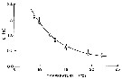
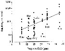
 Issued from : G.A. Deevey in Bull. Bingham Oceanogr. Coll., 1960, 17 (2); [p.76, Table IX]. Issued from : G.A. Deevey in Bull. Bingham Oceanogr. Coll., 1960, 17 (2); [p.76, Table IX].
Correlation coefficients for mean cephalothorax lengths for Paracalanus parvus with the temperature at sampled and averaged for the previous month from the English Channel (data from Digby, 1950).. |
| | | | Loc: | | | Cosmopolite (except Arctic), Antarctic (Indian), Beagle Channel, Magallones region, sub-Antarct. (SW Atlant., Indian, SW & SE Pacif.), Benguela Current, South Africa (E & W), Saldanha Bay, Atlant. (tropical, temperate), Argentina (mainly coastal, shelf, shelfbreak), Bahia Blanca, Peninsula Valdés, Mar del Plata, Uruguay (continental shelf), Brazil (off Rio de Janeiro, Guanabara Bay, Campos Basin, Cabo Frio, Vitoria Bay, Vitoria-Cabo de Sao Tomé, Mucuri estuary), Caribbean Colombia, Caribbean Sea, Jamaica (Kingston Harbour), G. of Mexico, Aransas Ship Channel, Angola (Baia Farta), G. of Guinea, Ivorian shelf, Casamance, Morocco-Mauritania, Cap Ghir, Canary Is., Chesapeake Bay, Narragansett Bay, Long Island Sound, Massachusetts Bay, Georges Bank, Emerald Bank, off SE Nova Scotia, Newfoundland, Labrador, S Davis Strait, SW Iceland, Ireland, Celtic Sea, Bristol Channel, English Channel, Roscoff, Morlaix estuary, Granville, Pas de Calais, Barents Sea (rare), Wyville Thomson Ridge (60°N), Norwegian Sea, Norway (Malangen fjord, Raunefjorden, Nordvestbanken, Hakøybotn, Kosterfjorden), NE Scotland, North Sea, Dogger Bank, Kattegat, Skagerrak, Gullmar Fjord (58°15'N, 11°26'E), Bay of Kiel, Bay of Lübeck, Gulf of Mecklenburger, off Madeira, Portugal (Mondego estuary, shelf); NW Spain,Bay of Biscay, Arcachon Bay, Gironde estuary, La Pallice roadstead, Belon estuary, Bilbao & Urdaibai estuaries, Santander, off Coruña, Vigo, off W Cape Finisterre, Portugal, Mondego Estuary, Ibero-moroccan Bay, off W Tangier, Medit. (M'Diq, Alboran Sea, Habibas Is., Sidi Fredj coast, El Kala shelf, Alger, laguna Mar Menor, Baleares, Banyuls, Berre Lagoon, Toulon Harbour, Villefranche-sur-Mer, Ligurian Sea, Tyrrhenian Sea, Napoli, Lake Faro (Sicily), Straits of Messina, NW Tunisia, Sfax, G. of Gabes, Malta, Adriatic Sea, Mljet Is., Venice, mouth of Po, G. of Trieste, Ionian Sea, Aegean Sea, Thracian Sea, Lebanon Basin, Iskenderun Bay, Haifa Bay, Bay, W Egyptian coast, Alexandria, Marmara Sea, Black Sea, Black River estuary, Sebastopol), Suez Canal, Lake Timsah, Shatm El-Sheikh, Taba, Hurghada, Safâga, Red Sea, Gulf of Oman, E South Africa (Natal), Arabian Sea, Arabian Gulf, UAE coast, Somalia, ? Maldive Is., Madagascar, India (Saurahtra coast, Bombay, Mangalore coast, Pointcalimere, Lawson's Bay, Porto Novo, Madras, Gulf of Mannar, Vellar estuary, Palk Bay, Rushikulya estuary, Mandarmani), Bay of Bengal, ? Nicobar Is., ? S Burma, Perai River estuary (Penang), Straits of Malacca, G. of Thailand, Malaysia (Sarawak: Bintulu coast), SW Celebes, Pacif. (tropical, sub-tropical), China Seas (Bohai Sea, Yellow Sea, East China Sea, South China Sea, Xiamen Harbour, Jiaozhou Bay, N Yangtze Riv. estuary), Taiwan Strait, Taiwan (S, E, SW, W, NW, N, NE, Mienhua Canyon), Hong Kong, Okinawa, S, E & W Korea (Chunsu bay, Muan Bay, Asan Bay, Seomjin River estuary, Yongsan River estuary), Geumo Is., Geoje Is., Japan Sea, Japan, Tokyo Bay, Yatsushiro-kai, Ariake-kai, Tsushima Straits, Japan (Kuchinoerabu Is., Nagazaki, Onagawa, Fukuyama, Seto Inland Sea, south estuaries, W Hokkaido), Oyashio region, off Sanriku, off Shikoku Is., Station Knot, Okhotsk Sea, Kurile Is., Bering Sea, British Columbia, Vancouver Is., Nitinat Lake, Dabob Bay, off Washington coast, Oregon (Yaquina Bay, off Newport), California, Los Angeles, La Jolla (San Diego), W BaJa California, Bahia Magdalena, Gulf of California, La Paz, Acapulco Bay (rare), G. of Tehuantepec, W Costa Rica, Pacif. (E equatorial), Clipperton Is., Bahia Cupica (Colombia), Peruvian coast & shelf, Chile (N, Mejillones Bay, off Valparaiso), Pacif. (W equatorial), New Caledonia, New Zealand (Kaikoura, off SE), Australia (SE), S Tasmania, Straits of Magellan, Ushuaia | | | | N: | 666 ? | | | | Lg.: | | | (7) F: 1-0,84; (14) F: 0,98-0,78; M: 0,99-0,85; (22) F: 1,3-0,74; M: 1,4-0,8; (28) F: 0,77-0,63; (34) F: 0,9-0,72; (35) F: 1,02-0,75; M: 1,02-0,82; (36) F: 1,18-1,02; M: 1,08; (38) F: 1,05-0,72; (45) F: 1-0,75; M: 1-0,9; (54) F: 1,01-0,96; M: 1,04; (59) F: 1,2-0,7; M: 1,2-0,8; (66) F: 0,99-0,85 (in forma major; 0,7-0,69; M: 0,76 (in forma minor; (72) F: 1; (73) F: 1,03-0,89; M: 1,03-0,88; (86) F: 0,99-0,75; (114) F: 1,12-0,97; 0,94-0,89; (116) F: 0,86; M: 1; (131) F: 1,3-0,7; M: 1,4-0,74; (142) F,M: 1,2-0,8; (145) F: 1,3; M: 1,4; (178) F: ? 0,8-0,68; 1-0,92; (180) F: 0,74-0,99; M: 0,79-0,9; (187) F: 1,1-1; (237) F: 0,75-1,1; M: 1,0-0,95; (322) F: 0,8; M: 0,75; (327) F: 1,17-0,86; M: 1,21-0,91; (335) F: 0,94-0,91; M: 0,92-0,88; (351) F: 0,9-0,98; M: 0,8-0,9; (354) F: 0,94-0,82; M: 1,02-0,82; (373) F: 1,07-0,86; M: 1,14-0,91; (432) F: 1,1-0,79; (449) F: 1-0,8; M: 1-0,91; (530) F: 0,9; M: 0,8; (786) F: 0,95-0,9; (795) F: 0,629; M: 0,5; (920) F: 0,91; (991) F: 0,7-1,2; M: 0,8-1,4; (1185) F: (1302) F: 0,622-0,852; M: 0,683-0,790; (1125) F: 1,0; (1185) F: 0,72-0,68; M: 0,92-0,78; {F: 0,62-1,30; M: 0,50-1,40}
The mean female size is 0.914 mm (n = 82; SD = 0.1658), and the mean male size is 0.957 (n = 48; SD = 0.1963). The size ratio (male : female) is 1.054 (n = 28; SD = 0.850). The males are generally slightly more large than females. | | | | Rem.: | épi-bathypélagique.
Sampling depth (Antarct., sub-Antarct.) : 100 m.
Généralement côtière et néritique, parfois en eau saumâtre.
Certaines confusions sont possibles avec P. indicus et P. quasimodo (Cf. Hiromi, 1987; Kang, 1996), doù certaines identifications peu sûres.
Corral Estrada (1970, Pl.13) représente une P4 plus proche de la P3 de P. indicus que deP. parvus (voir la présence de petites épines sur le bord distal externe de Exo 3 ).
Certaines localisations sont à confirmer, en particulier dans l'Indien et le Pacifique.
Observé dans les ballasts des navires à San Francisco.
Les figures données par Giesbrecht (1892), notamment la P5, semble bien correspondre à celle de Sars.
Voir aussi les remarques en anglais | | | Dernière mise à jour : 28/10/2022 | |
|
|
 Toute utilisation de ce site pour une publication sera mentionnée avec la référence suivante : Toute utilisation de ce site pour une publication sera mentionnée avec la référence suivante :
Razouls C., Desreumaux N., Kouwenberg J. et de Bovée F., 2005-2025. - Biodiversité des Copépodes planctoniques marins (morphologie, répartition géographique et données biologiques). Sorbonne Université, CNRS. Disponible sur http://copepodes.obs-banyuls.fr [Accédé le 03 décembre 2025] © copyright 2005-2025 Sorbonne Université, CNRS
|
|
|
|


;)
;)
;)
;)
;)
;)
;)
;)
;)
;)
;)
;)
;)
;)
;)
;)
;)
;)
;)
;)
;)
;)
;)
;)
;)
;)
;)
;)
;)
;)
;)
;)
;)
;)
;)
;)
;)
;)
;)
;)
;)
;)
;)

;)
;)
;)
;)
;)
;)
;)
;)
;)
;)
;)
;)
;)
;)
;)
;)
;)
;)
;)
;)
;)
;)
;)
;)
;)
;)