|
|
 |
Fiche d'espèce de Copépode |
|
|
Calanoida ( Ordre ) |
|
|
|
Diaptomoidea ( Superfamille ) |
|
|
|
Acartiidae ( Famille ) |
|
|
|
Acartia ( Genre ) |
|
|
|
Acanthacartia ( Sous-Genre ) |
|
|
| |
Acartia (Acanthacartia) tonsa Dana, 1849 (F, M) | |
| | | | | | | Syn.: | Acartia giesbrechti Dahl, 1894 c (p.13, 22, Rem.: Mouth of the Tocantins River, in the lower salinities 5.69 to 34.5 p.1000); Steuer, 1915; 1923 (p.23, figs.F,M); Björnberg, 1963 (p.66, Rem.);
? Acartia bermudensis Esterly, 1911 b (p.224, figs.F,M); Owre & Foyo, 1967 (p.101, figs.F,M);
? Acartia floridana Davis, 1948 (p.82, figs.F,M);
Acartia tonsa cryophylla Björnberg, 1963 (p.64, figs.F,M);
Acartia gracilis Herrick, 1887;
Acartia tonsa s.l. : Brinton & al., 1986 (p.228, Table 1);
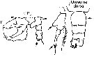
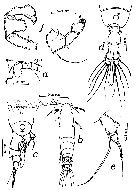
Acartia spp. : Hansen B.W. & al., 2016 (p.131, embryonic strain); Hansen B.W. & al., 2017 (p.984, pH effects). | | | | Ref.: | | | Giesbrecht, 1892 (p.508, 522, 770, figs.F,M); Giesbrecht & Schmeil, 1898 (p.154); Wheeler, 1901 (p.183, figs.F,M); Esterly, 1905 (p.204, figs.F,M); Sharpe, 1910 (p.414, fig.F); Steuer, 1923 (p.23, figs.F,M); Esterly, 1924 (p.105, figs.F,M); Remy, 1927 a (p.171, figs.F,M, Rem.); Wilson, 1932 a (p.160, figs.F,M); Rose, 1933 a (p.276, figs.F,M); Redeke, 1934 (p.39, figs.F, Rem.); Davis, 1944 (p.3); Farran, 1948 a (n°12, p.3, figs.F); Brodsky, 1950 (1967) (p.426, figs.F,M); Carvalho, 1952 a (p.152, Rem.M); ); Conover, 1956 (p.156 & suiv., figs.N, juv.); Anraku & Omori, 1963 (p.118, figs. mouth parts); Vervoort, 1964 a (p.24); 1965 (p.198, Rem.); Bowman, 1965 (p.150: Rem.); Gonzalez & Bowman, 1965 (p.257, figs.F,M, Rem.); Faber, 1966 p.191, fig.N); Ramirez, 1966 (p.19, figs.F,M); Marques, 1966 (p.10); Vidal, 1968 (p.41, figs.F,M); Pallares, 1968 b (p.29, figs.F, M); Ramirez, 1969 (p.84, fig.F, Rem.); Shih & al., 1971 (p.31); Arcos, 1975 (p.23, figs.F,M); Kos, 1976 (Vol. II, figs.F,M, Rem.); Dawson, 1979 (1980) (p.1, figs.F,M); Dawson & Knatz, 1980 (p.8, figs.F,M); Miller & al., 1980 (p.349, figs. Md: F, juv.V); Brylinski, 1981 (p.255, figs.F,M, carte); Björnberg & al., 1981 (p.661, figs.F,M, Rem.); Sazhina, 1982 (p.1160, Rem., fig.N); Schnack, 1982 (p.89, figs.Mx2, Md, Mxp); Montu & Gloeden, 1982 (p.361, anomalies); Gaudy & Vinas, 1985 (p.227); Sazhina, 1985 (p.83, figs.N); Zamora-Sanchez & Gomez-Aguirre, 1986 (p.339, figs.F,M, Rem.); Blades-Eckelbarger, 1991 (p.262, fig.F); Sabatini, 1990 (p.53, figs.juv.1-5, F,M); Belmonte & al., 1994 (p.9, figs.F,M); Garmew & al., 1994 (p.149, Rem.); Mazzocchi & al., 1995 (p.65, figs.F,M, Rem.); Hassett & Blades-Eckelbarger, 1995 (p.59, fig., 3, gut morphology, gut cells, digestive activities); Behrends & al., 1997 (p.594, figs.F); Hoffmeyer & Prado Figueroa, 1997 (p.257, figs.); Chen & Marcus, 1997 (p.587, Rem: uf); Belmonte, 1998 a (p.38, fig., Rem.: Eggs); Bradford-Grieve, 1999 (n°181, p.5, figs.F,M); Barthélémy, 1999 (p.858, 864, figs.F); 1999 a (p.9, Fig.23, K-M); Bradford-Grieve & al., 1999 (p.886, 962, figs.F,M); Castro-Longoria, 2001 (p.225, fig.4); Prusova & al., 2002 (p.65, figs.F,M); Caudill & Bucklin, 2004 (p.91: genetic diversity); Giesecke & Gonzalez, 2004 (p.607, fig.: Md); G. Harding, 2004 (p.24, figs.F,M); Ferrari & Dahms, 2007 (p.63, 71, Rem., Table VIII); Avancini & al., 2006 (p.115, Pl. 83, figs.F,M, Rem.); Vives & Shmeleva, 2007 (p.428, figs.F,M, Rem.); Drillet, Goetze & al., 2008 (p.109, genetic analysis, eggs); Chen G. & Hare, 1998 (p.1451, cryptic diversification); Chen & Hare, 2011 (p.2425, genetic); Harvey J.B.J. & al., 2012 (p.60, Table 2, molecular sequences); Laakmann & al., 2013 (p.862, figs.1, 2, 3, 5, Table 1, 2, molecular Biology); Blanco-Bercial & al., 2014 (p.5, 6: Rem.: problematic taxa); Jørgensen & al., 2019 (p.1440, genome, mRNA, genome size evolution). | 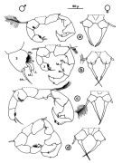 issued from : J.M. Brylinski in J. Plankton Res., 1981, 3 (2). [Fig.2, p.257]. Structure of P5 of the Acartia in the wet docks of the harbour of Dunkirk (Strait of Dover). Male and Female a: Acartia clausi; b: A. tonsa, c: A. discaudata, d: A. bifilosac.f.: curved finger, c.n.: curved needle, d.t.: distal tooth, l.: lamella, l.p.: lamellar process, p.t.: proximal tooth, s.: setae, sp.: spines, 3, segment 3 of left leg.
|
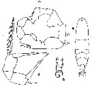
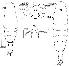
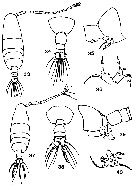
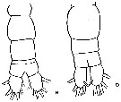
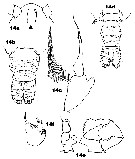
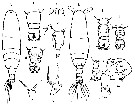
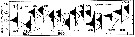
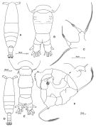 Issued from: M.G. Mazzocchi, G. Zagami, A. Ianora, L. Guglielmo & J. Hure in Atlas of Marine Zooplankton Straits of Magellan. Copepods. L. Guglielmo & A. Ianora (Eds.), 1995. [p.67, Fig.3.7.1]. Female: habitus (dorsal); B, urosome (dorsal); C, P5. Nota: Proportional lengths of urosomites and furca 46:16:18:20 = 100. Male: D, habitus (dorsal); E, urosome (dorsal); F, P5. Nota: Proportional lengths of urosomites and furca 16:29:18:8:14:15 = 100. Remarks: Both females and males of this species are hightly variable in the ornamentation of the urosomal somites. The specimens from Straits of Magellan resemble those described by Björnberg (1963) as A. tonsa var. cryophylla due to the remarkably reduced ornamentation of the urosome.
|
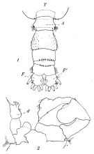
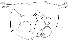
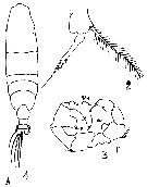
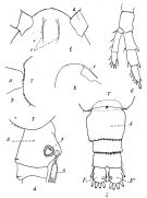 issued from : P. Remy in Annales de Biologie Lacustre, 1926 (1927 a), XV. [p.172, Fig.I]. Female (from Ouistreham): 1, forehead (ventral), r = rostral filaments; 2, idem (lateral); 3, last thoracic segment (T) and 1st urosomal segment (A); 4, idem (lateral right side), s = seminal receptacle, S = spermatophore; 5, urosome (dorsal), F & F' = caudal rami; 6, P4.
|
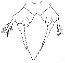
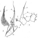 issued from : P. Remy in Annales de Biologie Lacustre, 1926 (1927 a), XV. [p.173, Fig.II]. Female (from Ouistreham): P5 (lateral view), (b = basal part; d = spinules; f = seta; m = muscles; p = lamellar process); 2, P5 (anterior view) (A and A' = basal segments).
|
 issued from : P. Remy in Annales de Biologie Lacustre, 1926 (1927 a), XV. [p.175, Fig.III). Male: 1, urosome (dorsal) (1 = genital somite; F & F' = caudal rami); 2, P5 (anterior view) (d = distal segment of left leg).
|
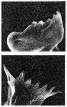
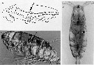
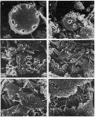
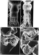 Issued from: M.G. Mazzocchi, G. Zagami, A. Ianora, L. Guglielmo & J. Hure in Atlas of Marine Zooplankton Straits of Magellan. Copepods. L. Guglielmo & A. Ianora (Eds.), 1995. [p.68, Fig.3.7.2]. Female (SEM preparation): B, urosome (dorsal), with a rows of small spinules on genital somite; C, detail of inner posterior margins of last thoracic somite (dorsal); D, urosome (lateral right side), with spermatophore attached to genital somite.; E, detail of spermatophore; F, P5; G, detail of distal end of P5. Bars: B, D 0.050; C, E, G, 0.010 mm.
|
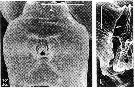
Issued from: M.G. Mazzocchi, G. Zagami, A. Ianora, L. Guglielmo & J. Hure in Atlas of Marine Zooplankton Straits of Magellan. Copepods. L. Guglielmo & A. Ianora (Eds.), 1995. [p.69, Fig.3.7.3]. Female (SEM preparation): B, urosome (dorsal); C, idem (ventral); D, P5 (posterior); E, right P5; F, detail of last segment of left P5. Bars: B, C 0.050 mm; D, E, F 0.010 mm.
|
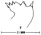
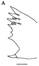 issued from : Giesecke & Gonzalez in Rev. Chil. Hist. Nat., 2004, 77. [p.610, Fig. 2 A]. Schematic drawing of the cutting edge of the left mandible blade of Acartia tonsa from Mejillones Bay, Chile . Mean (SD: standard deviation in parenthesis) Itoh's edge index: 896 (43), n = 14 specimens. Scale bar = 0.010 mm. Based on the Itoh index, the species belong to
|
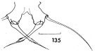 issued from : F.C. Ramirez in Contr. Inst. Biol. mar., Buenos Aires, 1969, 98. [p.80, Lam. XVI, fig.135 ]. Female (from off Mar del Plata): 135, P5. Scale bar in mm: 0.05.
|
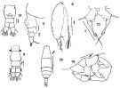 issued from : F.C. Ramirez in Bol. Inst. Biol. Mar., Mar del Plata, 1966, 11. [Lam.VI, Figs.8-14] Female (from off Mar del Plata): 8, habitus (lateral right side)10, P5; 11, urosome (lateral left side); 12, idem. Male: 9, urosome (dorsal); 13, habitus (dorsal); 14, P5.
|
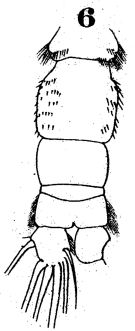 issued from : W. Giesbrecht in Fauna Flora Golf. Neapel, 1892, 19. [Taf.43, Fig.6]. Male: 6, urosome (dorsal).
|
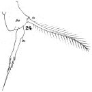
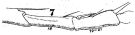 issued from : W. Giesbrecht in Fauna Flora Golf. Neapel, 1892, 19. [Taf.30, Fig.7]. Male: 7, right A1 (segments 18 and 19-21).
|
 issued from : W. Giesbrecht in Fauna Flora Golf. Neapel, 1892, 19. [Taf.30, Fig.24]. Female: 24, P5.
|
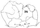 issued from : W. Giesbrecht in Fauna Flora Golf. Neapel, 1892, 19. [Taf.30, Fig.34]. Male: 34, P5.
|
 issued from : C.O. Esterly in Univ. Calif. Publs Zool., 1924, 26 (5). [p.106, Fig. N). Female (from San Francisco Bay): 1, forehead (lateral); 2, A1 (ventral); 3, forehead (ventral); 4, outline of posterior margin of thorax, to show spines; 5, margin of thorax and genital segment (lateral); 6, outline of posterior margin of thorax (lateral); 7, genital segment (ventral); 8, terminal part of Mxp; 9, habitus (lateral); 10, idem (dorsal); 11, urosome (lateral); 12, P4; 13, P3; 14, P2; 15, P1; 16, A2 (ventral); 17, 17-18, P5 (from side,; different specimens); 19, Md (citting edge); 20, P5. Nota: Relative lenfths of abdominal segments and caudal rami 11:4:2:5. 1st and 2nd abdominal segments with row of small teeth on posterior border
|
 issued from : C.O. Esterly in Univ. Calif. Publs Zool., 1924, 26 (5). [p.107, Fig. O). Male: 1, forehead (lateral); 2, urosome (dorsal); 3, habitus (dorsal); 4, grasping A1; 5, last thoracic and 1st abdominal segments; 6-7, outline of margin of last thoracic segment (lateral; different individuals) to show spines; 8, urosome (dorsal) from differnt specimen than in 2; 9, P1; 10, P5 (right foot at left); 11, end segment of left P5 (from a second specimen); 12-13, outlines of margin of last thoracic segment in two individuals, to show spines (lateral); 14, Segments of A1 proximal and distal to geniculation (proximal one at left); 15, terminal portion of Mxp; 16, urosome and margin of last thoracic segment (lateral). Nota: Relative lengths of abdominal segments and caudal rami 22:32:18:6:9:15. 1st segment with tuft of hairs on each side; row of delicate hairs each side of last segment; posterior, dorsal margin of 2nd to 4th with row of small teeth which, in second, extend along sides.
|
 issued from : C.O. Esterly in Univ. Calif. Publs Zool., 1905, 2 (4). [p.204, Fig.49]. Female (from San Diego Bay): a, habitus (dorsal); d, P5. Male: b, urosome (dorsal); c, P5 (dx = right foot).
|
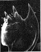 issued from : C.B. Miller, D.M. Nelson, R.L. Guillard & B.I. Woodward in Biol. Bull., 1980, 159 [p.350, Fig.1]. Scanning electron micrograph by A. Cornell-Bell. Female (from NW Atlantic: Vineyard Sound, Massachusetts): Mandibular gnathobase of adult reared at 12.6 microMol silicic acid. V = ventral tooth; C1 = large central tooth; C2 = smaller central tooth; L = limit of siliceous caps; N = nonsiliceous dorsal spine. Black bar represents 10 microns. Nota: A. tonsa has three siliceous teeth: a curving spine on the ventral end of the tooth list (V), a heavy crown with four rounded points in the center (C1), and a small bifurcate tooth just to right of center (C2). A. tonsa successfully extracted silicic acid from concentrations in seawater. Formation of normal teeth required concentration of 0.8 microMol or above. Copepodites and adults formed teeth at all of the silicic acid levels tested. However, typical specimens from low silicic-acid levels had teeth much lower in relief than those from high silicic-acid levels. This reduction was most evident in specimens from the 0.18 to 0.3 microMol concentrations. Reduction of teeth in specimens reared at low levels was variable both among individuals and among teeth on the same mandible. In a number of cases the ventral tooth was so reduced that in the SEM there appeared to be a hole completely through the siliceous structure to the chitin or tissue underneath (see Figure 2).
|
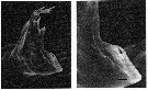 issued from : C.B. Miller, D.M. Nelson, R.L. Guillard & B.I. Woodward in Biol. Bull., 1980, 159 [p.356, Fig.2]. SEM by A. Cornell-Bellbr. Female: (Left figure) mandibular gnathobase of adult (reared at 0.22 microMol. silicic acid. The reduced ventral tooth is on the lower right. (Right figure) Detail of same jaw shows the character of the apparent hole in the ventral tooth. The black bar represents 2.5 microns.
|
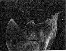 issued from : C.B. Miller, D.M. Nelson, R.L. Guillard & B.I. Woodward in Biol. Bull., 1980, 159 [p.357, Fig.3]. SEM by A.H. Soeldner. Female: Mandibular gnathobase of adult reared at 0.27 microMol. silicic acid. The central tooth shows severe reduction (the ventral tooth is at left). The black bar represents 5 micons.
|
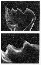 issued from : C.B. Miller, D.M. Nelson, R.L. Guillard & B.I. Woodward in Biol. Bull., 1980, 159 [p.358, Fig.4]. SEM by A.H. Soeldner. Female: (Above) Mandibular gnathobase from adult reared at 0.21 microMol. silicic acic. Both teeth show substantial, but not severe reduction. The ventral tooth is io the right. (Below) detail of central tooth shows the proximal-to-distal grooves usually on the surfaces of the teeth. The black bar represents 2.5 microns.
|
 issued from : C.B. Miller, D.M. Nelson, R.L. Guillard & B.I. Woodward in Biol. Bull., 1980, 159 [p.360, Fig.5]. SEM by A.H. Soeldner. Stage V: (Above) Mandibular gnathobase from copepodite reared at 0.21 microMol silicic acid. Both V and C1 show extreme reduction. (Below) Mandibular gnathobase from another copepodite reared at 0.21 microMol silicic acid. Neither V or C1 shows much wear. The black bars represents 5 microns. Nota: There is substantial reduction in one specimen, but not in other. Both the reduction and its variability occur in the younger stages as well as in adults.
|
 issued from : D.F.R. Arcos in Gayana, Zool., 1975, 32. [Lam.IX, Figs.71-74]. Female (from Bahia de Concepcion, Chile): 73, habitus (dorsal); 74, P5. Male: 71, habitus (dorsal); 72, P5.
|
 issued from : R.-M. Bathélémy in J. Mar. Biol. Ass. U.K., 1999, 79. [p.861, Fig.4, K, L]. Scanning electon miccrograph. Female: K, genital double-somite (ventral); L, detail of the right genital slit. Scale bars: 0.030 mm (K); 0.005 mm (L). Symbols: * = cuticular protuberance; arrowhead = lamellar flap; small arrow = genital slit.
|
 issued from : G. Harding in Key to the adullt pelagic calanoid copepods found over the continental shelf of the Canadian Atlantic coast. Bedford Inst. Oceanogr., Dartmouth, Nova Scotia, 2004. [p.24]. Female & Male. Nota: Female P5 basis with round process, apical segment not evenly tapered, toothed at center (arrowed). Male left P5 apical segment with two digitiform appendages; right penultimate segment with no spines on process (arrowed)
|
 issued from : T.K.S. Björnberg in Bol. Inst. Oceanogr. Sao Paulo, 1963, XIII, 1. [p.65, Fig.34]. As Acartia tonsa var. cryophylla. Female (from S Brazil): a, forehead; b, habitus (dorsal); c, last thoracic segment and urosome with spermatophore (right lateral); e, P5. Male: d, last thoracic segment and urosome (dorsal); f, P5. Nota: The abdomen of the female shows no spinulation along the margin of the abdominal segments; The P5 female have a longer marginal seta on the basal segment than the typical A. tonsa. The specimen is an indicator of cold southern water, therefore the name of the Brazilian new variety cryophylla (Salinity: 25.48-33.22 p.1000; temperatures: 14.38-15.40°C)
|
 Ma. E. Zamora-Sanchez & S. Gomez-Aguirre in An. Inst. Univ. Nal. Auton. Mexico, 56 (1985), Ser. Zool. (2), 1986. [Pl.3, p.344]. Female (from Laguna de Agiabampo, Golf of California): 33, habitus (dorsal); 34, last thoracic segment and urosome (dorsal); 35, last thoracic segment and genital segment (lateral); 36, P5 (dorsal view). Male: 37, habitus (dorsal); 38, last thoracic segment and urosome (dorsal); 39, last thoracic segment and urosomal segments 1-4 (lateral); 40, P5.
|
 issued from : J.K. Dawson in Harbors Environmental Projects, Univ. Southern California, 1979. [p.9, Fig.3]. Female (from Los Angeles Harbors): P5.
|
 issued from : J.K. Dawson in Harbors Environmental Projects, Univ. Southern California, 1979. [p.7, Fig.1]. Male: P5.
|
 issued from : J.K. Dawson in Harbors Environmental Projects, Univ. Southern California, 1979. [p.15, Fig.9, B, D]. Female : D, urosome (dorsal). Male: B, urosome (dorsal).
|
 issued from : B.W. Hansen, G. Drillet, M.F. Pedersen, K.P. Sjøgreen & B. Vismann in J. comp. Physiol. B, 182. [p.616, Fig.1]. Subitaneous eggs of Acartia tonsa exposed to abrupt and substantial changes in salinity. The eggs were transferred from normal salinity (32 psu) to 0 or 72 psu. At zero salinity : A vitelline coat and chorion shell; B perivitelline space; C egg plasma membrane and D embryo. Nota: When eggs kept at salinity 32 psu were abruptly exposed to hypo-saline conditions (0 psu), they swelled from about 80-90 micrometers in diameter, but they never exploded and they never hatched. Exposure of eggs to small, gradual changes in salinity was followed by changes in egg diameter and volume. The eggs exposed to 60 and 70 psu seawater imploded within 10 min whereas eggs exposed to 50 psu imploded after approximately 6 h. After C.R, trancription from conductivity (psu) to ClNa: psu valor x 0.58; and conductivity to total salts: psu x 0.65.
|
 issued from : R.P. Hassett & P. Blades-Eckelbarger in Mar. Biol., 1995, 124. [p.60, Fig.1 partial] Acartia tonsa (from Long Island Sound, New York). a, digestive system (drawn from digitized sagittal section) showing location of B-cells (arrowed). 1-3 midgut zones following terminology of Arnaud & al., 1978, e : aesophage; b-c, side and dorsal views, respectively, of adult female using differential interference contrast light microscopy, showing outline of gut epithelial layer and location of B-cells (arrowed)
|
 issued from : M. Anraku & M. Omori in Limnol. Oceanogr., 1963, 8. [p.122, Fig. 7, F] Acartia tonsa (from Woods Hole): Cutting edge of Md. Nota: The species has teeth of a somewhat different shape; some are sharp, others rounded.
|
 Issued from : J.M. Bradford-Grieve in ICES Identification Leaflets for Plankton N°181, 1999 [p.11, Figs.14 a-f]. Female: a, forehead (ventral) with rostral filaments; b, urosome (dorsal); c, P5. Male: d, urosome (dorsal); e, P5; f, exopodal segments 2+3 of left P5.
|
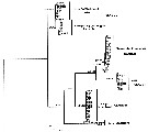 Issued from : K.G. da Costa, M. Vallinoto & R.M. da Costa in J. Coastal Res., 2011, SI 64. [p.362, Fig.2]; Phylogenetic ML tree based on 100 pseudore^licas of bootstrap. Numbers represent ML/MP/IB. Nota: The phylogenetic analyses produced similar tree topologies for all methods used, therefore, only the maximum likelihood tree is presented in the figure . The consensus tree has 5 clades: Clade I is composed of samples from Florida, and his the sister group of Clade II, which is made up of Chen & Hare's (2008) F-haplotypes from Chesapeake Bay. These clades are the sister group of Clade III (samples from Europe and Rhode Island), followed by Clade IV (Taperaçu, N Brazil) and Clade V (Chen & Hare's S haplotypes from North America). Most of these clades are supported by high boostrap values, although the relationships between clades are not well-supported. The Shimodaira-Hasegawa test was used to examine different constrained topologies. Genetic divergence btween the Taperaçu samples and the other clades varied between 21.6 % or 12.4 % (Clade III) and 28.7 % or 16.7 % (Clade I), according to the corrected and p distances respectively. However, including the outgroup , Acartia hudsonica (Ahu), these values increased to 37.8-47.7 % and 22.1-23.9 %. The authors in the discussion (p.361) note that the identification of cryptic species has increased mainly because of the increasing availability of DNA sequencing technology (see Bickford & al., 2006). Acartia tonsa is a widespread estuarine copepod, although recent studies of populations from the northwestern Atlantic and Europe have shown that the taxon may, in fact, represent a complex of cryptic species (see in Caudill & Bucklin, 2004; Drillet & al., 2008). While the species is cosmopolitan, these studies were restricted to North American and European populations. The present study has identified what appears to be a new cryptic A. tonsa species from northern Brazil. The specimens analysed were highly genetically distinct from those of their counterparts recorded from other sites. Chen & Hare (2008) interpreted the divergence between S and F haplotypes as evidence of species-level differentition rather than an ancestral polymorphism. These divergent mtDNA haplotypes are also supported by a nuclear marker (ITS). The degree of divergence is typical of that found between recognized copepod species (see Bucklin & al., 2003; Chen & Hare, 2008). No clear phylogeographic pattern was found in the present study, although additional analyses based on sequences with a relatively fast evolutionary rate may provide further insights. irrespective of possible geographic patterns, the profound divergence among the clades indicates a multiple, and thus ancient origin of these cryptic species. Using a 2% mutation rate, Chen & Hare (2008) concluded that the F and S lineages (clades II and V) split some 3.4 million years ago. As a similar degree of divergence was observed between these lineages and the Taperaçu clade, it seems reasonable to conclude that they also split at around the same time. This indicates that the present-distribution of the species of the A. tonsa complex has been determined by ancient vicariant events.
|
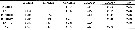 Issued from : K.G. da Costa, M. Vallinoto & R.M. da Costa in J. Coastal Res., 2011, SI 64. [p.361, Table 1]; Genetic divergence between the samples used in the present study. P distance is presented, while corrected distance under the diagonal. Nota: A 522 bp fragment of the mtCOI gene was obtained from specimens of Acartia tonsa collected in the Taperacu estuary in Bragança (N Brazil). The sequences were aligned with a database obtained from GenBank, which included those of Europe and North America. Two distinct haplotypes were identified. According to the AIC, the best-fit model of evolution was the K81uf+1 model (invariable site 0.6697), which was used to estimate genetic divergence.
|
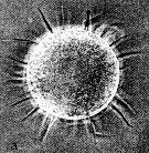 Issued from : N.H. Marcus in Mar. Biol., 1990, 105. [p.415, Fig.2, a]. Egg of Acaertia tonsa from sediment (coast of northern California, in February-April 1989). Egg diameter (µm); 80.6 ± 1.8 (N = 10) (sediments, February); 81.0 ± 0 (sediments, April); 81.4 ± 1.8 (spawned, February). Nota:: Egg surface with spines (spine lengths ranged from 18 to 25 µm)..
|
 Issued from : M.G. Mazzocchi in Guida al Riconoscimento del plancton dei Mari Italiani, Vol. II, 2006. [p.91, Tav. 83]. After A. Comaschi. Female: a, forehead with rostral filaments ((ventral); b, habitus (dorsal); c, urosome (dorsal); d, same); e, last thoracic segment and urosome with spermatophore (lateral); f-g, left P5 (various aspects). Male: h, habitus (dorsal); i-l, urosome (dorsal); m, P5; n, exopodal segments 2 + 3 (Re2+3) of left P5.
|
 Issued from : M.S. Kos in Field guide for plankton. Zool Institute USSR Acad., Vol. II, 1976. After Giesbrecht, 1892. Female: 1, habitus (dorsal); 2, P5. male: 3, P5.
| | | | | Ref. compl.: | | | Esterly, 1917 (p.393, light-dark reactions); 1919 (p.1, 16, light-dark reactions); Sewell, 1948 (p.392, 461); Conover, 1956 (p.156, biology); Grice, 1956 (p.50); Deevey, 1956 (p.126, 127, tab. IV); Conover, 1959 (p.259, Table 1, 2, respiration); Deevey, 1960 (p.5, Table II, fig.8, 13, 14: annual abundance, Rem.: p.25, fig.18, 19) ; Bowman, 1961 (p.206, Rem.); H. Schulz, 1961 (p.57); Wickstead, 1962 (p.546, food & feeding); Marshall & Orr, 1962 (tab.1, 3); Grice & Hart, 1962 (p.287, table 3); Fagetti, 1962 (p.37); Cervigon, 1962 (p.181, tables: abundance distribution); Ahlstrom & Thrailkill, 1963 (p.57, Table 5, abundance); Gaudy, 1963 (p.29, Rem.); Anraku, 1964 a (p.221, grazing, predation); 1964 b (p.195, respiration-grazing vs. temperature); Lance, 1965 (p.155, Table 1, 2, respiration vs osmotic pressure); Martin, 1965 (p.185, 188: Table 1); Heinle, 1966 (p.59, P/B quotient); Faber, 1966 a (p.418, 419); Fleminger, 1967 a (tabl.1); Bishop, 1967 (p.23, predators); Subbaraju, 1967 (p.18, developmental time vs latitude); Hargrave & Geen, 1968 (p.332, phosphorus excretion); Emery, 1968 (p.293, swarm); Vinogradov, 1968 (1970) (p.106); Mullin, 1969 (p.308, Table I: estimates of production); Heinle, 1969 (p.186, temperature effect); 1969 a (p.150, Table 1, culture); 1970 (p.360, population dynamics); Itoh, 1970 a (p.8: tab.2); Reeve, 1970 (p.894, Rem.: p.901); Reeve & Cosper, 1970 (p.1, temperature effect); Wilson D.F. & Parrish, 1971 (p.202, mating); Zillioux & Gonzalez, 1972 (p.217, egg dormancy); Björnberg, 1973 (p.354, 384); Heinrich, 1973 (p.95, fig.1); Arndt & Heidecke, 1973 (p.599, 603); Mullin & Evans, 1974 (p.902, efficieny in food chain); Wilson D.S., 1974 (p.909, food size selection); Arashkevich, 1975 (p.351, fig.2, digestion time); Anderson G., 1975 (p.747, parasited by epidarid isopod); Peterson & Miller, 1975 (p.642, 650, Table 3, interannual abundance); Corkett & Zillioux, 1975 (p.13, temperature vs egg laying); 1976 (p.14, Table 1, 2, 3, abundance vs. interannual variations); Uye & Fleminger, 1976 (p.253, resting egg, hatching); Grahame, 1976 (p.219, Table X); Arcos, 1976 (p.85, Rem.: p.97); Roman, 1977 (p.149, feeding); Peterson & Miller, 1977 (p.717, Table 1, seasonal occurrence); Miller & al., 1977 (p.326, growth); Ikeda, 1977 b (p.29, respiration rate); Richman & al., 1977 (p.69, grazing: particle selection); Reeve & Walter, 1977 (p.211, grazing vs food concentrations); Allan & al., 1977 (p.317, grazing); Honjo & Roman, 1978 (p.45, fecal pellet, sinking rate); Parrish & Wilson, 1978 (p.65, fecundity); Knatz, 1978 (p.68, Table 1, fig.3, abundance, %); Lee & McAlice, 1979 (p.228, annual cycle); Lonsdale & al., 1979 (p.235, carnivorous behavior); McAlice, 1981 (p.267, post-glacial history); Grice & Marcus, 1981 (p.125, Dormant eggs, Rem.: p.130, 135, 136); Cahoon, 1981 (p.1215, reproductive rate vs. food quality); Bartram, 1981 (p.25, feeding vs development); Arashkevich & al., 1982 (p.477, Table 2, diet); Citarella, 1982 (p.791, 798: listing, frequency, fig.5, Tableau II, V); Turner & Dagg, 1983 (p.16); Landry, 1983 (p.614, development times vs. stages); Durbin & al., 1983 (p.1199, size-weight, Chl a, egg production); ); Roman, 1984 (p.949, feeding); Stearns & Forward, 1984 (p.85, photosensiivity); 1984 a (p.91, photobehavior); Turner, 1984 b (p.265, Table 1, fig.3-7: pellet contents); Dussart, 1984 (p. 25, 62:,occurrence); Tremblay & Anderson, 1984 (p.3); Peterson, 1985 (p.726, fig.2, abundance); Donaghay, 1985 (p.235, food quality, egg production); Stoecker & Sanders, 1985 (p.85, grazing); Tester, 1985 (p.45, egg-hatching); Baars & Oosterhuis, 1985 (p.71, Table 4: gut passage time); Kiørboe & al., 1985 (p.85, metabolism, egg production, respiration); Ambler, 1985 (p.743, egg production vs. seasonal factors); 1986 (p.183, egg production); Stearns, 1986 (p.65, grazing behavior); Sullivan & McManus, 1986 (p.121, resting egg production); Beckman & Peterson, 1986 (p.917, egg production); Støtrup & al., 1986 (p.87, fig. 2, 3, Table 1, 2, cultivation as food for fish larvae); Buskey & al., 1986 (p.65, behavior); Stoecker & Egloff, 1987 (p.53, feeding); Stearns & al., 1987 (p.305, grazing); Houde & Roman, 1987 (p.229, ingestion vs food quality); Libourel Kiørboe & Tiselius, 1987 (p.525, gut clearance); Johansen & Møhlenberg, 1987 (p.137, toxicity/egg production); Peterson W.T. & Bellantoni, 1987 (p.411, Table I, figs.7 egg production vs. total chlorophyll concentration); Bellantoni & Peterson, 1987 (p.199, egg production); Jimenez-Perez & Lara-Lara, 1988 (p.122); Kleppel & al., 1988 (p.185, gut contents); Paffenhöfer & Stearns, 1988 (p.33, clearance rate); Dagg, 1988 (p.167, egg production vs. physical event); Donaghay, 1988 (p.469, acclimatation vs. food quality & trophic dominance); Berggreen & al., 1988 (p.341, food size spectra, feeding, growth, production); Daan & al., 1988 (p.45, Table 4, carnivorous behaviour); Turner & Tester, 1989 (p.21, grazing); Tester & Turner, 1989 (p.231, feeding rate); Verity & Smayda, 1989 (p.161, ingestion-egg production); White & Dagg, 1989 (p.315, egg production vs. suspended sediment); Citarella, 1989 (p.123, abundance); Stearns & al., 1989 (p.7, egg production); Cervantes-Duarte & Hernandez-Trujillo, 1989 (tab.3); Sabatini, 1989 (p.847, annual cycle); Farabegoli & al., 1989 (p.207, occurrence ); Marcus, 1990 (p.413, tab.1, fig.2: egg); Støttrup & Jensen, 1990 (p.87, feeding, egg production); Tester & Turner, 1990 (p.169, Fig.4); Stoecker & McDowell Capuzzo, 1990 (p.891, feeding); Jonsson & Tiselius, 1990 (p.35, feeding behaviour, prey detection); Durbin & al., 1990 (p.23, diel feeding behavior); Mallin, 1991 (p.481); Haigh & Taylor, 1991 (p.301, Rem.: p.309); Zagami & Guglielmo, 1990 (p.71, 1st occurrence); Fransz & al., 1991 (p.10); Gifford, 1991 (p.8, Table 2, diet); Gifford & Dagg, 1991 (p.161, feeding); Fernandez Araoz, 1991 (p.575); Tester & Turner, 1991 (p.603); Lee B.-G & Fisher, 1992 (p.117, fecal pellets); Huntley & Lopez, 1992 (p.201, Table 1, A1, B1, eggs, egg-adult weight, temperature-dependent production, growth rate); Hirche, 1992 (p.395, Table 1, egg production, r-strategy); Durbin & al., 1992 (p.342, Table 5, size-weight, egg production); White & Roman, 1992 (p.239, egg production); Kleppel, 1992 (p.57, feeding); Arfi & al., 1992 (p.213, filtration rate); Kimmerer, 1993 (tab.2); Roman & al., 1993 (p.1603, Oxygen effect); Saiz & al., 1993 (p.280, predation effect); Cervetto & al., 1993 (p.1207, feeding, respiration, egg production); Snell & Carmona, 1994 (p.255); Marcus & Lutz, 1994 (p.83, hatching success vs. anoxia); Lutz & al., 1994 (p.119, hatching/O2 effect); Jonasdottir, 1994 (p.67, nutrition vs reproduction); Belmonte & al., 1994 (p.9, occurrence vs. Black Sea); Miller & Marcus, 1994 (p.235, sinking velocity eggs); Wieser, 1994 (p.1, Rem.: p.18, fig.4A); Hoffmeyer, 1994 (p.303); Suarez Morales, 1994 b (tab.1); Butler & Dam, 1994 (p.81, production rates fecal pellets); Saiz & Kiørboe, 1995 (p;147, feeding modes and turbulence effect); de Angelis & Lee, 1994 (p.1298, methane production); Hajderi, 1995 (p.542, 1st occurrence); Santos & Ramirez, 1995 (p.133, Tabl. I, fig.2, 3); Tiselius & al., 1995 (p.369, feeding behaviour and reproduction between field and laboratory); Madhupratap & al., 1996 (p.77, Table 2: resting eggs); Marcus, 1996 (p.143); Hansen B. & Bech, 1996 (p.257, bacteria associated); Hansen B. & al., 1996 (p.275, degradation fecal pellets); Diaz Zaballa & Gaudy, 1996 (p.1123, seasonal variations); Kiørboe & al., 1996 (p.65, feeding: prey switching behaviour); Lenz & al., 1996 (p.1, behaviour); Ban S, Burns C. & al., 1997 (p.287, Table 1, 2, feeding, reproduction); Tiselius & Jonsson, 1997 (p.164, predation); Marcus & al., 1997 (p.291, hatching success vs. anoxia); Mauchline, 1998 (tab.15, 16, 17, 18, 19, 21, 22, 23, 24, 25, 26, 33, 35, 36, 38, 40, 45, 46, 47, 48, 51, 53, 54, 56, 58, 62, 63, 64, 66, 68, 69, 78, fig.66); Lopes & al., 1998 (p.195); Alvarez-Cadena & al., 1998 (tab.2, 3); Hopcroft & al., 1998 (tab.2); Feinberg & Dam, 1998 (p.87, fecal pellets vs diet); Suarez-Morales & Gasca, 1998 a. (p107); Lavaniegos & Gonzalez-Navarro, 1999 (p.239, Appx.1); Gomez-Gutiérrez & Peterson, 1999 (p.637, Table II, abundance); Cervetto & al., 1999 (p.33); Buskey & al., 1999 (p.995, isotope C variations); Onishchik, 1999 (p.76); Harvey & al., 1999 (p.1, 49: Appendix 5, in ballast water vessel); Støttrup & al., 1999 (p.257, development, lipids vs. algal diets); Escribano & Hidalgo, 2000 (p.283, tab.2); Gaudy & al., 2000 (p.51, metabolism, temperature & salinity effects); Camatti & al., 2000 (p.41); Alvarez-Silva & Gomez-Aguirre, 2000 (p.163: tab.2); Gubanova, 2000 (p.105, introduction); Tester & al., 2000 (p.418, toxicity); Hidalgo & Escribano, 2001 (p.159, tab.2); Hidalgo & Escribano, 2001 (p.157, fig.4); Fransz & Gonzalez, 2001 (p.255, tab.1); Belmonte & Potenza, 2001 (p.174, 175: Rem.); Ara, 2001 b (p.121); Peterson & al. (p.381, Table 2, interannual abundance); Bressan & Moro, 2002 (tab.2); Uysal & al., 2002 (p.17, tab.1); Viñas & al., 2002 (p.1031); Besiktepe & Dam, 2002 (p.151, ingestion & defecation vs diet); Thor & al., 2002 (p.296, diet vs carbon incorporation); Dunbar & Webber, 2003 (tab.1); Zagorodnyaya & al., 2003 (p.52); Gubanova, 2003 (p.94, 99); Peterson & Keister, 2003 (p.2499, interannual variability); Vieira & al., 2003 (p.S163, Table 2, abundance); Titelman & Kiørboe, 2003 a (p.137, nauplius behaviour); Buskey & Hartline, 2003 (p.28, behaviour, escape response); Broglio & al., 2003 (p.267, feeding, reproduction vs. prey fatty composition); Krumme & Liang, 2004 (p.407, tab.1); Ara, 2004 (p.179, figs. 3, 4, 5); Marrari & al., 2004 (p.667, tab.1); Vargas & Gonzalez, 2004 (p.151); Gaudy & Verriopoulos, 2004 (p.219): Invidia & al., 2004 (p.187, egg vs. anoxia and sulfide vs pH); Gomes & al., 2004 (p.941, vertical migration vs. stratified waters); Gubanova, 2005 (p.146); Alvarez-Silva & al., 2005 (p.39); Choi & al., 2005 (p.710: Tab.III); David & al., 2005 (p.171); Berasategui & al., 2005 (p.485, tab.1); Manning & Bucklin, 2005 (p.233, Table 1); Bagøien & Kiorboe, 2005 a (p.129, mating vs. hydromechanical signal); Holste & Peck, 2005 (p.1061, egg production, hatching success vs. temperature & salinity); Azeiteiro & al., 2005 (p.7, fig.2, table 2, dynamic, production); Frangoulis & al., 2005 (p.254, Table I: C/N/P fecal pellet composition); Berasategui & al., 2006 (p.485: fig.2); Marques & al., 2006 (p.297, tab.III) ; Lopez-Ibarra & Palomares-Garcia, 2006 (p.63, Tabl. 1, seasonal abundance vs. El-Niño, Rem.: p.74); Roman & al., 2006 (p.435, nutrition); Sterza & Fernades, 2006 (p.95, Table 1, occurrence); Sei & Ferrari, 2006 (p.1, occurrence); Sei & al., 2006 (p.121, feeding, eggs viabiliity vs. oxygenation); Escribano, 2006 (p.20, Table 1); Hooff & Peterson 2006 (p.2610); Nielsen P. & al., 2006 (p.171, hatching success vs anoxia); Papastephanou & al., 2006 (p.3078, Table 3); Selifonova, 2006 (p.117); Drillet & al., 2006 (p.714, egg vs. cold storage); Camatti & al., 2006 (p.46, fig.5); Oppert, 2006 (p.1, diet vs. oxygen % , life history); Holste & Peck, 2006 (p.1061, egg production vs temperature, salinity, photoperiod, stocking density); Sørensen & al., 2007 (p.84, Rem.: eggs); David & al., 2007 (p.59: tab.2); Woodson & al., 2007 (p.163: Rem; behavior); Speekmann & al., 2007 (p.759); Pedroso & al., 2007 (p.173, silver toxicity); S.C. Marques & al., 2007 (p.213, Table 1, fig.6); Chojnacki & al., 2007 (p.45, Table 2); Biancalana & al., 2007 (p.83, Tab.2, 3); Sullivan & al., 2007 (p.259, Rem.: climate change); Leandro & al., 2007 (p.215); Pinho & al., 2007 (p.62); Youn & Choi, 2007 (p.222: Table1, egg production); Castro & al., 2007 (p.486, fig.3, Table 1, 2, 3); Morales C.E. & al., 2007 (p.452, Rem.: p.462: abundance); David & al., 2007 a (p.429, figs.2, 4, 5, 6, Table 3, 4, 5, 6); Marques S.C. & al., 2007 (p.725, Table 1, fig.4, climate variability); Titelman & al., 2007 (p.1023, Table I, Rem: mating); Jepsen & al., 2007 (p.764, adult density vs. egg production); Putland & Iverson, 2007 (p.173, eclogy); Sullivan & al., 2008 (p.485); Chen & Hare, 2008 (p.1451, molecular biology, cryptic ecological diversification); Smith J.R. & al., 2008 (p.937, Rem.: feeding behavior); Ayon & al., 2008 (p.238, Table 4: Peruvian samples); Peck & al., 2008 (p.102, egg production); Shmeleva & al., 2008 (p.31, Table 1); Waggett & Buskey, 2008 (p.111, Table 1); Muelbert & al., 2008 (p.1662, Table 1); Calliari & al., 2008 (p.18, salinity effecs); Hubareva & al., 2008 (p.131, Table 1, 2); Saco-Alvarez & al., 2008 (p.275, Table 1, toxicity from fuel tanker); Drillet, Jepsen & al., 2008 (p.47, life history of 4 strains); Tiselius & al., 2008 (p.93, reproduction, biomass, mortality); Larsen & al., 2008 (p.47, fig.1, Table 1, swimming-temperature-viscosity); Galbraith, 2009 (pers. comm.); Calliari & al., 2009 (p.1045, grazing, egg production rates); Brylinski, 2009 (p.253: Tab.1, p.256: Rem.); Ohs & al., 2009 (p.114, Rem.: eggs); Tartarotti & Torres, 2009 (p.106, UV effects); Kozlowsky-Suzuki & al., 2009 (p.395, Table 2, nutrition, oocyte development); Aravena & al., 2009 (p.621, seasonal & spatial distribution vs environmental factors); Telesh & al., 2009 (p.18: Table 2.1); Magalhaes & al., 2009 (p.187, Table 1, %); Escribano & al., 2009 (p.1083, Table 1, figs.6, 10); Primo & al., 2009 (p.341, Table1, interannual variations); Elliott & Tang, 2009 (p.585, dead/live vs staining); Hansen B.W. & al., 2010 (p.305 (egg hatching); C.E. Morales & al., 2010 (p.158, Table 1); Escribano & Pérez, 2010 (p.301, Fig.4: fatty acids); Hernandez-Trujillo & al., 2010 (p.913, Table 2); Hidalgo & al., 2010 (p.2089, fig.2, 4, Table 2, cluster analysis); Zenetos & al., 2010 (p.397); Yen & Lasley, 2010 (p.177, Rem.: p.183, mating): Mazzocchi & Di Capua, 2010 (p.423); Thor & Wendt, 2010 (p.1779, Carbon absorption); Medellin-Mora & Navas S., 2010 (p.265, Tab. 2); S.C. Marques & al., 2011 (p.59, Table 1, seasonal variability); Hogfors & al., 2011 (p.1460, fig.1, egg production); Acheampong & al., 2011 (p.151, egg production vs biochemical food), Rem: p.157, resting egg; Bollens & al., 2011 (p.1358, Table III); Kusk & al., 2011 (p.959, development vs environment & polluant); Magalhaes & al., 2011 (p.1520, seasonal abundance); Magris & al., 2011 (p.260, abundance, interannual variability); Escamilla & al., 2011 (p.379, spatial & seasonal abundance, competition); Costa R.G. da & al., 2011 (p.364, Table 1, seasonal occurrence); Tutasi & al., 2011 (p.791, Table 2, abundance distribution vs La Niña event); Scheef & Marcus, 2011 (p.363, resting eggs); Buskey & al., 2011 (p.57, fig.3, sensory perception vs predator); Gemmell & Buskey, 2011 (p.1773, nauplii/copepodites vs fish predation); Turner & al., 2011 (p.1066, Table II, abundance 1998-2008); Drillet & al., 2011 (p.831, feeding vs microbial preparation); Menéndez & al., 2011 (p.281, tidal effect); Ramos Avila & al., 2011 (p.323, chitobiase enzyme activity); Elliot & Tang, 2011 (p.1039, spatial & temporal distribution); 2011 a (p.1, population dynamics, mortality rate); Jiang & al., 2011 (p.947, resistance vs dinoflagellate); Saba & al., 2011 (p.291, harmful algal vs grazing); Bickel & al., 2011 (p.105, mortality vs turbulence); Amin & al., 2011 (p. 1965, clearance, feeding, egg production vs diets); Chen X. & al., 2011 (p.451, C N Fe concentration vs diet, egg production); Chen X. & al., 2011 (p.716, fatty acid vs diet); Alver & al., 2011 (p.100, nauplius stages); Saba & al., 2011 (p.47, excretion); Sichlau & al., 2011 (p.665, diapause eggs in sediments); Costa K.G. da & al., 2011 (p 356, fig. 2: phylogenetic tree, genetic divergence); Drillet & al., 2011 (p.2064, resting egg production vs food limitation); Postel, 2012 (p.327, Table 1, Fig.6); Delpy & al., 2012 (p.1921, Table 2); Hansen B.W & al., 2012 (p.613, eggs/salinity); Stefanova & al., 2012 (p.403, Table 2, interannual abundance); Olivotto & al., 2012 (p.685, egg production, molecular analysis); Guenther & al., 2012 (p.405, 411); Menéndez & al., 2012 (p.11, variability vs physical processes); Borg & al., 2012 (p.1, Nauplii swimming); Bruno & al., 2012 (p.1, Nauplii behaviour); Gorbi & al., 2012 (p.2023, test of toxicity vs eggs, nauplii); Malzahn & Boersma, 2012 (p.1408, feeding vs growth); Hong J. & al., 2012 (p.1, feeding behavior vs algal toxins); Drillet & al., 2012 (p.155, Table 1, culture); Kimmel & al., 2012 (p.76, long-term abundance record vs eutrophication); Muxagata & al., 2012 (p.475, Table 3, growth, annual production); Gonçalves & al., 2012 (p.321, abundance vs climatic variability); Menéndez & al., 2012 (p.389, Table 1: seasonal abundance); Spinelli & al., 2012 (p.39, potential prey for fish); Gonçalves & al., 2012 a (p.16, abundance, diel vertical behavior); Lavaniegos & al., 2012 (p. 11, Table 1, fig.3, seasonal abundance, Appendix); Buskey & al., 2012 (p.57, Fig.1, 3, behavior vs predator); Miyashita & al., 2012 (p.1557, Table 2: occurrence); Oechsler-Christensen & al., 2012 (p.161, grazing vs phytoplankton pigments); Aguirre & al., 2012 (p.341, Table I: abundance vs season, figs.4, 7); Durbin & al., 2012 (p.72, feeding & digestion rates); Hidalgo & al., 2012 (p.134, Table 2, 3, figs.5, 6, spatial distribution vs hydrology); Takahashi M. & al., 2012 (p.393, Table 2, water type index); Gusmao & al., 2013 (p.279, Table 4, sex ratio); Gubanova & al., 2013 (in press, Rem.: p.5, Table 4, fig.2, alien species); Palomares-Garcia & al., 2013 (p.1009, Table I, abundance vs environmental factors); in CalCOFI regional list (MDO, Nov. 2013; M. Ohman, pers. comm.); Gissi & al., 2013 (p.86, Table 3, copper toxicity); Chaalali & al., 2013 (p.1, abundance change vs. environmental conditions during the period 1992-2010); Elliott & al., 2013 (p.1027, low-oxygen effects); Elliott & al., 2013 a (p.1, hypoxia effects); Finiguerra & al., 2013 (p.17, sex tolerance vs. starvation); Hubareva & Svetlichny, 2013 (p.742, t° & Sal. tolerance); Garbosa da Costa & al., 2013 (p.756, Table 1, abundance vs tide); Zhang J. & al., 2013 (p.65, diets vs egg production, hatching success); Heuschele & al., 2013 (p.399, Table 2, mate behavior); Jarvis & al., 2013 (p.1264, Zinc oxide effects vs survival, production); Peijnenburg & Goetze, 2013 (p.2765, genetic data); Hansen B.W. & Drillet, 2013 (p.66, oxygen consumption, subitaneous and delayed hatching eggs); Fernandez-Severini & al., 2013 (p.1495, heavy metals concentrations); Alvarez-Silva & Torres-Alvarado, 2013 (p.241, Table1: seasonal abundance); Dunlap & al., 2013 (p.1375, mortality vs viral infestion); Mendoza Portillo, 2013 (p.37: Fig.7, seasonal dominance); Lidvanov & al., 2013 (p.290, Table 2, % composition); Pansera & al., 2014 (p.221, Table 2, abundance); Rice & al., 2014 (p.23, fig.3, size vs years 1952-2011); Pino-Pinuer & al., 2014 (p.83, Table 1, fig.3, 4, abundance variation vs time); Fierro Gonzalvez, 2014 (p.1, Tab. 3, 5, occurrence, abundance); Ortega & al., 2014 (p.495, Table I); Hylander & al., 2014 (p.149, figs. 2, 3, Table 2; life history vs UV exposure); Derisio & al., 2014 (p.197, occurrence vs turbidity); Drillet & al., 2015 (p.3028, eggs); Jepsen & al., 2015 (p.420, cultivation vs ammonia); Ruz & al., 2015 (p.200, seasonal abundance vs egg production, hatching success vs O2); Fuentes-Reinés & Suarez-Morales, 2015 (p.369, Table 1, Rem. p.373); Meunier & al., 2016 (p.50, selective feeding vs N/P contents for nauplii, copepodite); Wendt & al., 2016 (p.871, antifouling toxicity); Uriarte & al., 2016 (p.718, abundance vs years, climate change); Escribano & al., 2016 (p.1, growth rate); Araujo & al., 2016 (p.1, Table 3, abundance, %); Ben Ltaief & al., 2017 (p.1, Table III, Summer relative abundance); El Arraj & al., 2017 (p.272, table 2, spatial distribution); Ortega & al., 2017 (p.123, fig. 1, 5, 6, table 2, abundance, %); Trottet & al., 2017 (p. 7, Table 3: resting stage); Marques-Rojas & Zoppi de Roa, 2017 (p.495, Table 1); Atique & al., 2017 (p.1, Table 1, fig.8, Rem.: p.11); Jerez-Guerrero & al., 2017 (p.1046, Table 1: temporal occurrence); Buskey & al., 2017 (p.754, amyelinate fiber vs. escape response); Baumgartner & Tarrant, 2017 (p.387, resting eggs, fig.5, Rem.); Belmonte, 2018 (p.273, Table I: Italian zones); Nilsson & Hansen, 2018 (p.1, embryonic quiescence timing vs. embryos viability); Dias & al., 2018 a (p.189, fig.11: seasonal variation, Rem.: p.196); Palomares-Garcia & al., 2018 (p.178, Table 1: occurrence); Camatti & al., 2019 (p.1, fig. 3, 4, 5, 7, 8, 9, 10, Table 1, 2, 3, 4, 5, history of successful invasion); Richirt & al., 2019 (p.3, Table 1, fig.2, 3, 4, 5, abundance changes vs. years 1998-2014, table 2: diversity index); Acha & al., 2020 (p.1, Table 3: occurrence % vs. ecoregions, Table 5: indicator ecoregions). | | | | NZ: | 16 | | |
|
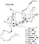
Carte de distribution de Acartia (Acanthacartia) tonsa par zones géographiques
|
| | | | | | | | | | | | | | | 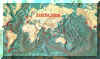 Carte de 1996 Carte de 1996 | |
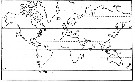 issued from : P. Remy in Annales de Biologie Lacustre, 1926 (1927 a), XV. [p.179]: geographic distribution in 1926. issued from : P. Remy in Annales de Biologie Lacustre, 1926 (1927 a), XV. [p.179]: geographic distribution in 1926.
1 : Port-Jackson (Australia) catches by Dana in 1840. 2 to 7: Pacific coast from South America (Valparaiso to Coquimbo and Arica, Chile; Mollendo and Callao, Peru) by Giesbrecht (1892). 8 and 9: Pacific coast from North America (San Diego region) by Esterly, 1905, 1923. 10: Bay of San Francisco by Esterly, 1924. 11: Sub-Antarct (Falkland Is.) by T. Scott, 1914. 12: Northwestern Atlantic (Mouth of Orenoque) by Cleve, 1900. 13, coast of Louisiane by Foster, 1904; 14-18:: Jamaica Bay near New York and along the coast until the bay of Fundy, by Sharpe (1910), Wheeler (1900), Williams (1906, 1907), Steuer (1923). 19-20: In the Indian Ocean (Mouth of Indus by Cleve, 1904; Maldive islands by Wolfenden, 1905. In Sunda Islands by, Cleve, 1901. In France (Channel of Caen-Ouistreham harbour)
|
 issued from : J.M. Brylinski in J. Plankton Res., 1981, 3 (2). [p.256, Fig.1]. issued from : J.M. Brylinski in J. Plankton Res., 1981, 3 (2). [p.256, Fig.1].
Geographical distribution of Acartia tonsa in northern European waters. |
 issued from : M.E. Sabatini in Scient. Mar., 1989, 53 (4). [p.855, Tabl.2]. issued from : M.E. Sabatini in Scient. Mar., 1989, 53 (4). [p.855, Tabl.2].
Seasonal occurrence, number and duration of Acartia tonsa generations in different areas.
Locality; Latitude; temperature range (°C) ; seasonal occurrence; number of generations (cohorts); generation time (in weeks); author reference. |
 issued from : G.B. Deevey in Bull. Bingham Oceanogr. Coll., 1960 (2). [p.27, Fig.14]. issued from : G.B. Deevey in Bull. Bingham Oceanogr. Coll., 1960 (2). [p.27, Fig.14].
Variations in length (from the top of the head to the base of the caudal rami) of Acartia tonsa females and males in the Delaware Bay (NW Atlantic Ocean). |
 issued from : J.T. Turner in P. S. Z. N. I: Mar. Ecol., 1984, 5 (3). [p.273, Fig.5]. issued from : J.T. Turner in P. S. Z. N. I: Mar. Ecol., 1984, 5 (3). [p.273, Fig.5].
Contents of fecal pellets from Acartia tonsa females from Station A-2 (off Mississipi Eiver mouth) on 9 December 1981.
a and b: small unidentified centric diatom (arrow); c: fragments of Skeletonema costatum (S) and an uniddentified centric diatom (UC); d: fragments of an unidentified diatom; e: Chaetoceros sp. spine (C) and fragments of a crustacean exoskeleton (CE), note dagger-like spines which appear to be chemoreceptors; f: crustacean appendages (CA) underneath the pellet peritrophic membrane (PM). |
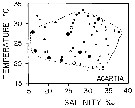 issued from : M.R. Reeve in Bull. mar. Sc., 1970, 20 (4). [p.902, Fig.4]. issued from : M.R. Reeve in Bull. mar. Sc., 1970, 20 (4). [p.902, Fig.4].
Temperature-salinity diagram for Acartia tonsa in Biscayne Bay (Florida, Miami). |
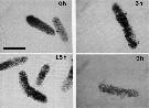 issued from : B. Hansen, F.L. Fotel, N.J. Jensen & S.D. Madsen in J. Plankton Res., 1996, 18 (2). [p.284, Fig.6, p.285, Fig.6 continued]. issued from : B. Hansen, F.L. Fotel, N.J. Jensen & S.D. Madsen in J. Plankton Res., 1996, 18 (2). [p.284, Fig.6, p.285, Fig.6 continued].
Video prints of the degradation of fecal pellets incubated in 0.22 micrometer filtered seawater as a function of time. The fecal pellets were produced on the nanoflagellate Rhodomonas baltica at excess food by the copepod Acartia tonsa.
The light intensity and video camera shutter speed were kept equal at all readings to make direct comparison possible. Scale bar = 0.100 mm.
Nota: Degradation of freshly produced fecal pellets in suspension was followed over time by volume recording and estimation of carbon loss.
The fecal pellets produced on a diatom diet were very dense and showed a significantly slower degradation than those produced on nanoflagellate or dinoflagellate diets. This indicates that the algal texture (i.e. the mechanical robustness given by inert structures) determines the degradation rate of the pellets.
The degradation rate was also very dependent on the algal concentration for the grazer (565 microgg. C per day T 1/2 = 75 h; excess food T 1/2 = 12 h).
Disintegration and degradation are processes of bacterial activity and mechanical stress in combination while the fecal pellets are in a suspension with no predators (see Jacobsen & Azam, 1984). Fecal pellets, in situ, however, are presumably exposed to coprophagy and coprorhexy from mesozooplankton (see Noji & al., 1991). The authors found a faster degradation while ciliates (Euplotes sp.) were accidentally contaminants in an incubation vial.
Free-living bacteria colonized the fecal pellets. After initiating colonization, the bacteria penetrated the peritrophic membrane, wich clearly leaked out material, observed as fecal pellets losing color (fig.6). Then the bacteria began the degradation of the fecal pellet matrix (Noji & al., 1991; Gonzalez, 1992). This scenario was already suggested by Gowing & Silver (1983) and Dellile & Razouls (1994) who stated that fecal pellets generally contain abundant internal bacteria.
During the degradation of the diatom-based pellets, the authors frequently observed coprochaly, where the matrix of the pellets swells, with the content of labile carbon disappearing. This was, however, never observed in the present nanoflagellate and dinoflagellate experiments.
Corner & O'Hara (1986, p.303) underline that after Sochard & al. (1979) studying microorganisms in Acartia tonsa found a unique gut flora dominated by numerous species of the genus Vibrio, and Gowing & Silver (1983) found that the mean volumes of bacteria inside such pellets were greater than those on their surface, a condition still prevailing after these pellets had been aged for over five days in sea water. Honjo & Roman (1978) could detect no bacteria in the faecal pellets released by copepods fed on bacteria-free diets. |
 issued from : M.M. Mullin & P.M. Evans in Limnol. Oceanogr., 1974, 19 (6). [p.907, Fig.2]. issued from : M.M. Mullin & P.M. Evans in Limnol. Oceanogr., 1974, 19 (6). [p.907, Fig.2].
Biomasses (bodily carbon) of various components integrated over the water column in the deep tank (cylinder 10 m deep and 3 m in diameter, about 70 m3 of sea water [from the Scripps Institution, La Jolla, San Diego], fiiltered through fine diatomaceous earth; to darken during the experiment.
Arrows on the ababsissa indicate the start and end phases of the experiment. The dashed line under ''copepods'' indicates the biomasses of Acartia tonsa and Paracalanus parvus during the transition period.
Nota: Establishment of a linear food chain consisting of the chain-forming diatom Skeletonema costatum, the copepods A. tonsa and P. parvus (particle-grazing), and ultimately the ctenophore Pleurobrachia bachei (coastal carnivore).
The experiment was divided into three phases; during the first two phases only copepods were present, A. tonsa initially dominating but subsequently being replaced by P. parvus (phase II). Phase III was that portion of the experiment when ctenophores were present together with P. parvus.
Assuming that the C:Chl ratio was maintened in the deep tank, the contribution of phytoplankton to the total particulate carbon (fig.2) can be calculated. The median level of the remaining, presumably detrital, particulate carbon was 140 mg/m3 (similar to the concentration of detritus in the near surface waters off La Jolla).
During phase I, when Acartia was dominant, the biomass of copepods fluctuated considerably and then declined until Paracalanus became dominant, thus starting phase II. It appear that Paracalanus has a higher rate of turnover than does Acartia but uses its food supply less effectively, resulting in a slightly lower food chain efficiency.
The median biomass of ctenophores in the tank was 16% that of the copepods during phase III (fig.2) and the biomass of copepods was similar to the local biomass of prey species for Pleurobrachia in spring, summer and fall (see Hirota, 1974: Table 10).
The field study of a marine planktonic food chain with which the experiment's results can be most directly compared is that of Petipa & al. (1970) in the Black Sea. |
 Issued from : R.J. Conover in Bull. Bingham Oceanogr. Coll., 1956, XV. [p.181, Fig.13]. Issued from : R.J. Conover in Bull. Bingham Oceanogr. Coll., 1956, XV. [p.181, Fig.13].
Size distribution of adult females Acartia tonsa from Long Island Sound ( U.S.A.) at different times of the year, 1952-1953. |
 Issued from : R.J. Conover in Bull. Bingham Oceanogr. Coll., 1956, XV. [p.176, Fig.11, C]. Issued from : R.J. Conover in Bull. Bingham Oceanogr. Coll., 1956, XV. [p.176, Fig.11, C].
Seasonal distribution in percent of total organisms of adults and naupliiAcartia tonsa from Long Island Sound, U.S.A.) 1952-1953.
The number of generations was estimated from the distribution of nauplii and adults.
The nauplii of each generation are designated by Roman numerals and the corresponding adults in Arabic;
Nota: There were probably 4 generations annually in the Sound, produced in the period from June through March. The development ofhe first two generations is clear enough; however, on September 23, a secondary peak of adults appeared which must have produced some of nauplii III. After mid-October, the percentage of A. tonsa in the tows increased while totals of all species were decreasing, suggesting that tonsa was more resistant to fall and winter conditions than other summer zooplankton forms..
In any event, adult peak 3 appears to be significant. The designation IV applies to low levels of nauplii produced through the cooler months. Possibly a few of the early IV nauplii matured so as to produce an overwintering population which consisted of both adults 3 and 4 |
 Issued from : E.J. Buskey, P.H. Lenz & Hartline D.K. in Adaptative Behavior, 2012, 20 (1). [p.62, Fig.3]; Issued from : E.J. Buskey, P.H. Lenz & Hartline D.K. in Adaptative Behavior, 2012, 20 (1). [p.62, Fig.3];
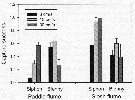
Comparison of capture success of the copepod Acartia tonsa by a predator mimic (siphon) and a fish predator, the coral reef blenny Acanthemblemaria spinosa at three different water speeds in a unidirectional paddle flume, or a slosh flume that simulates the oscillatory flow of surface waves.
Error bars represent standard error.
Data from Robinson & al., 2007 and Clarke & al., 2009
Nota: Althrough the maximum water speeds in the two fumes were similar, the reversing flow in the slosh flume produced much higher levels of turbulence compared with the continuous flow in the paddle flume. The different patterns of capture success (the proportion of copepods captured by the siphon or fish compared with the number of copepods encountered) demonstrated by the siphon and the fish, clarified the separate effects of water motion on the predator and its prey.
For both flume types, the capture success of the siphon increased with increasing flow speeds. However, capture success with the siphon was consistently higher in the slosh flume than in the paddle flume at comparable speeds, suggesting that the copepod had more difficulty recognizing the flow signal associated with the siphon in the more turbulent flows of the slosh flume.
When the disturbances are detected, copepods respond quickly with escape jumps that can accelerate them from a stationary position to speeds of over 600 body lengths per second within a few milliseconds. Myelinated nerves may improve the escape behavior of some copepods through faster conduction of nerve impulses. The differences in response latencies between myelinate and amyelinate copepod species are greatest in larger copepod species, where nerve signals must be conducted over longer distances.
Small amounts of turbulence favor the predator, while too much turbulence reduces predation. |
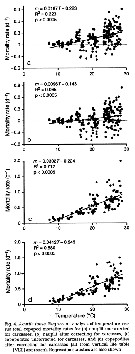
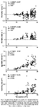
 Peterson W.T. & Bellantoni, 1987 (p.415, fig.6]. Peterson W.T. & Bellantoni, 1987 (p.415, fig.6].
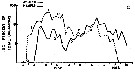
Fecundity of Acartia tonsa and Temora longicornis in Long Island Sound (USA). |
 Peterson W.T. & Bellantoni, 1987 (p.416, Fig.7, c, d]. Peterson W.T. & Bellantoni, 1987 (p.416, Fig.7, c, d].
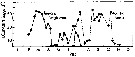
Scattergramms of egg production against chlorophyll concentration for Acartia tonsa in Long Island Sound.
The rates obtained with in situ temperatures > 17°C. Data from 30 October and 7 and 20 November shown in figure 6 are not included because low temperatures rather than food concentration probably limited fecundity on those days. |
 Issued from : T. Kiørboe, E. Saiz & M. Viitasalo in Mar. Ecol. Prog. Ser., 1996, 143. [p.68, Fig.1]. Issued from : T. Kiørboe, E. Saiz & M. Viitasalo in Mar. Ecol. Prog. Ser., 1996, 143. [p.68, Fig.1].
Acartia tonsa. Calm water functional response to variations in the concentration of diatoms: (A) ingestion and (B) clearance. (o) Diatoms Thalassiosira weissflogii only; (black o) T. weissflogii and ciliate Strombidium sulcatum added at a concentration of 12 ml per l. Error bars show ± SD.
Nota: The copepod Acartia tonsa has 2 different prey encounter stategies. It can generate a feeding current to encounter and capture immobile prey (suspension feeding) or it can sink slowly and perceive motile prey by means of mechanoreceptors on the antennae (ambush feeding). It is hypethesized taht A. tonsa adopts the feeding mode that generates the highest energy intake rate; i.e. that prey selection changes according to the relative concentration of alternative prey (prey switching) and that the copepod spend disproportionately more time in the feeding mode that provides the greatest reward. based on earlier observations , it is hypothesized that turbulencnce changes food selection towards motile prey. |
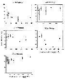
 Issued from : X. Chen, S.B. Baines & N.S. Fisher in Limnol Oceanogr., 2011, 56 (2). [p.455, Fig.2]. Issued from : X. Chen, S.B. Baines & N.S. Fisher in Limnol Oceanogr., 2011, 56 (2). [p.455, Fig.2].
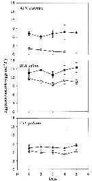
Egg production rates of Acartia tonsa feeding on Fe-replete (filled symbols) and Fe-depleted (open symbols) cells of (A) Thalassiosira oceanica, (B) Rhodomonas salina, (Diatoms), and (C) Isochrysis galbana (Prymnesiophyte), over a 5-d period.
Data points are means of 3 replicates ± 1 SD.
Nota: Egg production was always lower for copepods fed an Fe-depleted diet, regardless of the algal species that was used as food. When T. oceanica was used as a food source, the rate of egg production decreased significantly over 5-d feeding period in the low-Fe treatment, but in all other cases egg production dir not vary systematically over the course of the experiment.
After 5-d of feeding on T. oceanica, copepods produced eggs at a rate of 7.4 eggs per individual per day under Fe-replete conditions, and 0.6 eggs per ind. per day in the Fe-depleted treatment after 5 days of feeding..
When fed on Fe-replete R. salina and I. galbana the egg production rate after 5 days of feeding was 15.4 eggs per ind. per day and 8.5 eggs per ind. per day, respectively, while Fe-depleted R. salina and I. galbana diets at the same time resulted in egg production rates of 10.4 eggs per ind. per day and 6.2 eggs per ind. per day, respectively.
As noted by several authors, iron (Fe) is a limiting nutrient for phytoplankton growth in over 30 % of the world's oceans, including the Equatorial Pacific Ocean, the Southern Ocean, the Subarctic Pacific, and some coastal areas (see Martin & al., 1991; Hutchins & Bruland, 1998; Hutchins & al., 2002). Fe-deficient phytoplankton cells have lower nitrogen (N), phosphorus (P) and sulfur concentrations and higher silicon (Si) (Twining & al., 2004). |
 Issued from : X. Chen, S.B. Baines & N.S. Fisher in Limnol Oceanogr., 2011, 56 (2). [p.456, Fig.3]. Issued from : X. Chen, S.B. Baines & N.S. Fisher in Limnol Oceanogr., 2011, 56 (2). [p.456, Fig.3].
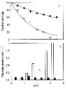
Naupliar survival of Acartia tonsa feeding on Fe-replete or Fe-depleted Thalassiosira oceanica (Diatom).
(A) Time series of number of surviving individuals for the Fe-depleted (open circles) and Fe-replete (filled circles) treatments. The lines represent best-fit regressions of the form Nt = 100 e -mt, where Nt is the number of individuals alive at time t, and m is the instantaneous mortality rate. The last two points for the Fe-depleted treatment (open circles with crosses) were not used to fit the lines because of elevated mortality rates during these periods.
(B) Time series of mortality rate for the Fe-depleted (open bars) and Fe-replete (filled rates). Mortality calculated as the fraction of individuals that died durung that interval divided by the number alive at the start of the interval.
Nota: All nauplii in the Fe-depleted treatment died within 1 week after hatching, whereas 60 % of the nauplii fed on Fe-replete diatoms survived during this period.
The daily mortality rate of nauplii fed on Fe-depleted T. oceanica was higner than for nauplii fed Fe-replete food for every 1-d interval during the experiment. Average instantaneous mortality estimatd by regression was 30 % ± 4 % per day when nauplii were fed Fe-depleted food and 8 % ± 0.4 % per day when fed Fe-replete food.
Carbon ingestion rates of algae ranged between 1.31 µg C per ind. per day and 3.01 µg C per ind. per day under all food conditions during the 5-d feeding period.. C ingestion rates were not affected by Fe status of algal food for any algal species. C ingestion rates of copepods ingesting T. oceanica were significantly higher than those feeding on R. salina and I. galbana, but no significant difference was observed between R. salina and I. galbana treatments. |
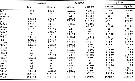
 Issued from : X. Chen, S.B. Baines & N.S. Fisher in Limnol Oceanogr., 2011, 56 (2). [p.457, Table 2]. Issued from : X. Chen, S.B. Baines & N.S. Fisher in Limnol Oceanogr., 2011, 56 (2). [p.457, Table 2].
Rates of Fe and C assimilation in copepods A. tonsa (µmol per ind. per day, µmol per ind. per day, respectively) fed on three species of algae. Values shown are means from 3 reolicate cultures ± 1 SD.
Nota: The rates of Fe and C assimilation in copepods fed on Fe-replete and Fe-depleted algal cells show that C assimilation was unaffected by the Fe content of the diet, but Fe assimilation was significantly greater (21-28 times) when copepods fed on Fe-replete cells than when fed Fe-depleted cells.
The Fe:C ratios in copepods that fed on Fe-replete cells (47.8 ± 7.9 (µmol per mol.) were not significantly different from Fe:C ratios in copepods that fed on Fe-depleted algae (54.8 ± 8.7 µmol per mol.) |
 Issued from : X. Chen, S.G. Wakeham & N.S. Fisher in Limnol Oceanogr., 2011, 56 (2). [p.721, Table 6]. Issued from : X. Chen, S.G. Wakeham & N.S. Fisher in Limnol Oceanogr., 2011, 56 (2). [p.721, Table 6].
Fatty acic concentration in Acartia tonsa after feeding on thhree different algal species (mg per g C) that had been grown under Fe-deficient and Fe-replete conditions. Means of duplicate samples ± variance. nd: not detected.
Nota Laboratory experiments to determine the influence of iron on the fatty acid and sterol composition of the diatom Thalassiosira oceanica, the cryptothyte Rhodomonas salina, the prymnesiophyte Isochrysis galbana, and the copepod Acartia tonsa that fed on these algae
Algal cells were cultured with no added Fe or with Fe added at 100 nmol per L.
Fe-deficient culture medium resulted in lower growth rates, cell volumes, and photosynthetic efficiencies for all algal species.
The btotal mass of fatty acid per cell was 2.2-3.1 times as high in Fe-replete cells as in Fe-deficient cells; on a carbon-normalized basis, the fatty acid concentrations of Fe-replete algal cells were 1.4-1.5 times as high.
Differences were noted between Fe treatments for specific satured, nonsaturated, and poluunsaturated fatty acid within each algal species.
Differences in lipid concentration and composition between Fe-replete and Fe-deficient algae may partly explain the lower egg production rate of copepods fed Fe-deficient algae. |
 Issued from : X. Chen, S.G. Wakeham & N.S. Fisher in Limnol Oceanogr., 2011, 56 (2). [p.721, Table 7]. Issued from : X. Chen, S.G. Wakeham & N.S. Fisher in Limnol Oceanogr., 2011, 56 (2). [p.721, Table 7].
Sterol concentrations in Acartia tonsa after feeding on three different algal species (mg per g C) that had been grown under Fe-deficient and Fe-replete conditions. Means of duplicate samples ± variance. nd: not detected. |
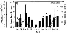
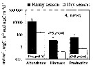 Issued from : A. Magalhaes, D.S.B. Nobre, R.S.C. Bessa, L.C.C. Pereira & R.M. da Costa in J. Coastal Res., 2011, SI 64. [p.1522, Fig.2]. Issued from : A. Magalhaes, D.S.B. Nobre, R.S.C. Bessa, L.C.C. Pereira & R.M. da Costa in J. Coastal Res., 2011, SI 64. [p.1522, Fig.2].
Seasonal variation in the abundance, biomass and productivity of Acartia tonsain the Taperaçu estuary (00°55'06.8''S, 46°44'00''W) in July (rainy season) and October (dry season), 2004, during spring tides (flood and ebb periods), at 3-hour intervals over 24-hour period. with a plankton net (300 µm mesh aperture). |
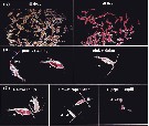
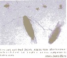 Issued from : D.T. Elliot & K.W. Tang in Mar. Ecol. Prog. Ser., 2011, 427. [p.1]. Issued from : D.T. Elliot & K.W. Tang in Mar. Ecol. Prog. Ser., 2011, 427. [p.1].
Acartia tonsa (from lower Chesapeake Bay, USA) live (red color) and dead (brown color) after treatment with neutral red stain showing individuals (nauplii in top row, copepodites in bottom row).
Nota: Mortality is a poorly constrained parameter in population dynamics. Uncertainty in mortality rate stems from the inherent difficulties in measuring this process in situ (see Ohman & Wood, 1995). A posteriori adjustments of mortality rates are required to match model predictions to observations (see Runge & al., 2004), because mortality can affect the behavior of population dynamics models and nutrient-phytoplankton models (see Steele & Henderson, 1992).
Studies of population dynamics have often focused on predatory mortality, to the exclusion of non-predatory factors. Several studies have considered non-predatory mortaliy due to factors such as physiological state, diet and starvation (reviewed in Carlotti & al., 2000), as well as disease and parasitism (see Kimmerer & McKinnon, 1990), environmental stressors (see Carpenter & al., 1974) and ageing (see Rodriguez-Graña & al., 2010). There is no a priori reason to consider in situ non-predatory mortality of marine copepods as negligible. An analysis of longevity data from field and laboratory studies suggested that non-predatory factors account for 25 to 33 % of total mortality among adult copepods in the sea (see Hirst & Kiørboe, 2002)
Non-predatory mortality leaves behind a carcass that, in an estuary, may remain in the water column for several days (see Tang & al., 2006 ; Elliot & al., 2010) in the open ocean it may remain for months (see Terazaki & Wada, 1988). Failure to identify carcasses in samples could skew estimates of live copepod abundance and associated ecological parameters. For example, if one were to estimate copepod production from abundance data on a single day, assuming that all collected animals were alive, the true production would br surestimated by a factor of (1/Plive) exp. G, where Plive is the proportion actually alive on that day and g is the number of generations over which the forecast is made.
Consider the estuarine A. tonsa, which may have 9 generations in a year (Mauchline, 1998), multiple years of field sampling have demonstrated that from about 10 to 30 % of individuals in the lower Chesapeake Bay are carcasses (see Tang & al., 2006 ; Elliott & Tang, 2011). Assuming a relatively consevative value of 15 % dead A. tonsa (i.e 85 % alive and producing), annual production foresasted from abundance data taken during the first generation of the growing season would be overestimated by a factor of (1/0.85) exp.9 = 4.32 if carcasses were counted as live copepods.
Elliott & Tang (2011) described the abundance of live copepods and carasses in the lower Chesapeake Bay over 2yr. Cacasses were identified by neutral red vital staining. The authors found that copepod carcasses were prevalent throughout the study area, and that visibly injured carcasses were rare (< 2% of carcasses). The majority of these carcasses appeared to have resulted from non-predatory mortality. |
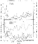
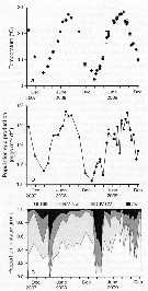 Issued from : D.T. Elliot & K.W. Tang in Mar. Ecol. Prog. Ser., 2011, 427. [p.4, Fig.1].Acartia tonsa Time series of (a) mean (diamonds) and range (bars) of water temperature, (b) mean temperature-specific population egg production rate predictions from equation of Holste & Peck, 2006 (Table 1), and (c) mean proportion observed in each developmental stage group (nauplii NI-NIII, NIV-NVI); copepodite CIV-CV; adult CVI) used to estimate mortality rates (copepodite CI-CIII not used). Means are from all samples within a specific tributary on a specific date. Issued from : D.T. Elliot & K.W. Tang in Mar. Ecol. Prog. Ser., 2011, 427. [p.4, Fig.1].Acartia tonsa Time series of (a) mean (diamonds) and range (bars) of water temperature, (b) mean temperature-specific population egg production rate predictions from equation of Holste & Peck, 2006 (Table 1), and (c) mean proportion observed in each developmental stage group (nauplii NI-NIII, NIV-NVI); copepodite CIV-CV; adult CVI) used to estimate mortality rates (copepodite CI-CIII not used). Means are from all samples within a specific tributary on a specific date.
Nota; After removing carcasses, instantaneous mortality rates for nauplii varied from <0.01 per day to a maximum of 0.35 per day and for copepodites from <0.01 per day in winter to 0.5 per day or higher in summer. Non-predatory mortality comprised an average of 25 % of total mortality for nauplii, and 12 % of total mortality for copepodites.. Predatory mortality alone was insufficient to keep yje population size under control during the growing season (from June to October), demonstrating the importance of non-predatory mortality in the lower Chesapeake Bay.
Total mortality rates varied in a cyclic manner annually, peaking in the summer. Corrected total mortality for nauplii varied from near 0.0 per day in the fall and spring to a maximum of 0.12 per day in June 2008 and 0.35 per day in August 2009.Corrected total mortality for copepodites was near 0.0 per day in the winter, and ca. 0.7 per day in summer 2008 and 0.9 per day in summer 2009, with a maximum of 1.52 per day in July 2009.
Corrected mortality rates were significantly different from uncorrected rates, both for nauplii and copepodites.
The difference was obvious for nauplii, where uncorrected mortality rates were consistently higher than corrected rates. Mortality rate estimates for copepodites were only slightly influenced by the inclusion of carcasses. This was due to the fact a similar percentage of carcasses was found in both CIV-CV and CVI copepodite stage groups, meaning that carcasses caused only a small bias in the abundance ratio that was used to estimate mortality by the vertical life table approach.
Water temperature predicted the vast majority of explained variation in mortality rates, being responsible for >98 % of each model R2 value. Water temperature varied cyclically during both years of study, with annual maxima near 28°C in July and August.
Predicted population egg production rate showed also an annual cycle, peaking in July through September, with lowest values in January of both years. Overall, estimated population egg production rates were consistently high (>1000 eggs per m3 per day) from April through October. The proportions of individuals in each developmental stage group were similar throughout most of the study period, except during winter when the relative abundance of adults increased markedly. Stage-duration-corrected abundancedeclined across consecutive stage groups during spring, summer, and fall,although only slightly between NI-NIII and NIV-NVI. Again, the exception was seen in winter samples when duration of NIV-NVI were higher than NI-NIII. |
 Issued from : D.T. Elliot & K.W. Tang in Mar. Ecol. Prog. Ser., 2011, 427. [p.7, Fig.4]. Issued from : D.T. Elliot & K.W. Tang in Mar. Ecol. Prog. Ser., 2011, 427. [p.7, Fig.4].
Acartia tonsa (from Chesapeake lower Bay, USA). Regression analysis of temperature vs total copepod mortality rates.
VLT approach: vertical life Table approach. see in Aksnes & Ohman, 1996. |
 Issued from : D.T. Elliot & K.W. Tang in Mar. Ecol. Prog. Ser., 2011, 427. [p.9, Fig.7]. Issued from : D.T. Elliot & K.W. Tang in Mar. Ecol. Prog. Ser., 2011, 427. [p.9, Fig.7].
Acartia tonsa (from Chesapeake lower Bay, USA). Regression analysis of temperature vs predatory and non-predatory mortality rates.
VLT approach: vertical life Table approach. see in Aksnes & Ohman, 1996. |
 Issued from : D.T. Elliott & K.W. Tang in Limnol. & Oceangr.: Methods, 7, 2009. [p.589, Fig.2]. Issued from : D.T. Elliott & K.W. Tang in Limnol. & Oceangr.: Methods, 7, 2009. [p.589, Fig.2].
Appearance of neutral red-trated zooplankton under stereomicroscope (Nikon SMZ1000- and recommended lightling. Shown are 100 % dead and 100 % live Acartia tonsa (A), patchily stained and pink individuals (B), and the live and dead individuals of various developmental stages (C). |
 Issued from : D.T. Elliott & K.W. Tang in Limnol. & Oceangr.: Methods, 7, 2009. [p.588, Table 2]. Issued from : D.T. Elliott & K.W. Tang in Limnol. & Oceangr.: Methods, 7, 2009. [p.588, Table 2].
Comparison of preservation methods on the % stained Acartia tonsa. |
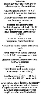 Issued from : D.T. Elliott & K.W. Tang in Limnol. & Oceangr.: Methods, 7, 2009. [p.587, Fig.1]. Issued from : D.T. Elliott & K.W. Tang in Limnol. & Oceangr.: Methods, 7, 2009. [p.587, Fig.1].
Diagram of the recommended protocol of the neutral red method for collection, staining, and live/dead sorting of zooplankton samples. |
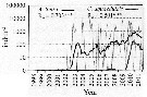 Issued from : I. Uriarte, F. Villate & A. Iriarte in J. Plankton Res., 2016, 38 (3). [p.724]. Issued from : I. Uriarte, F. Villate & A. Iriarte in J. Plankton Res., 2016, 38 (3). [p.724].
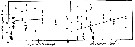
Monthly time-series from 1998 to 2011 of Acartia tonsa (black) and Calanipeda aquaedulcis (grey) in the inner estuary of Bilbao (NW Spain). Thicker lines are moving averages. Ro is the Spearman's rank correlation coefficient (***P<0.001).
Nota: From 2003 to 2009, a replacement in the dominance of indigenous neritic species (as Acarti clausi) by the newly arriving non indigenous brackish species Acartia tonsa occurred and showed a positive correlation with temperature and Secchi disk depth and negative correlation with streamflow.
Acartia tonsa were not observed in the inner estuary of Bilbao until 2002. By 2003, it had colonized this inner estuary becoming the dominant copepod and displacing the indigenous neritic congener A. clausi to the outer estuary. The species have been found to be able to inhabit low oxygen waters (see Roman & al., 1993; Marcus & al., 2004; Itoh & al., 2011) although severe hypoxia can cause lethal effects. |
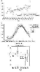 Issued from : E. Rice, H.G. Dam & G. Stewart in Estuaries and Coasts, 2014. [p.17, Fig.2, A, B; Fig.3, C]. Issued from : E. Rice, H.G. Dam & G. Stewart in Estuaries and Coasts, 2014. [p.17, Fig.2, A, B; Fig.3, C].
A: Inshore Central Basin of Long Island Sound trend of temperature over 1978-2012. Correlation coefficient (tau) = 0.49, p <<0.01. Line shownh is the best fit, slope = 0.03, intercept = -43.2. N = 63. Data from the NOAA Milford Laboratory.
B: Off shore surface temperatures for Central Basin stations (mean and 2SD) for 1994-2012 and reported values from Riley & al. (1986) for 1952-1954.
C: Box-and-whisker plot of mean prosome lengths (µm) of Acartia tonsa in August, September and November 1952, 2010, and 2011. The thick, center line in each box represent the first and third quartiles, respectively; dashed lines represent the range; and open circles are outlies. |
 Issued from : P.M. Ruz, P. Hidalgo, S. Yàñez, R. Escribano & J.E. Keister in J. Mar. Syst., 2015, 148. [p.208, Fig.6]. Issued from : P.M. Ruz, P. Hidalgo, S. Yàñez, R. Escribano & J.E. Keister in J. Mar. Syst., 2015, 148. [p.208, Fig.6].
Temporal changes of female abundance (Ln number per m3), egg abundance (number per L) and egg production rate in situ samples (EPR) (Ln eggs per female per day) for Acartia tonsa in Mejillones Bay (23°S, 70°25'W). |
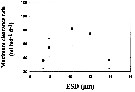 Issued from : S. Besiktepe & H. G. Dam in Mar. Ecol. Prog. Ser., 2002, 229. [p.155, Fig.2]. Issued from : S. Besiktepe & H. G. Dam in Mar. Ecol. Prog. Ser., 2002, 229. [p.155, Fig.2].
Acartia tonsa. Maximum clearance rate (mean ± SD, n= 6to 10) versus mean food particle equivalent spherical diqmeter (ESD). Each ESD corresponds to a different diet (see Table 1).
Copepods cultured in the laboratory, from eggs of females collected from Long Island Sound (USA). |
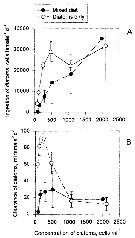
 Issued from : S. Besiktepe & H. G. Dam in Mar. Ecol. Prog. Ser., 2002, 229. [p.153, Table 1]. Issued from : S. Besiktepe & H. G. Dam in Mar. Ecol. Prog. Ser., 2002, 229. [p.153, Table 1].
Summary of diets and concentrations used in experiments of Acartia tonsa. ESD = equivalent spherical diameter. Values in parentheses are standard deviation of triplicate replicates. NMFS = National Marine Fisheries Service; CT: Connecticut; LIS = Long Island Sound; WHOI = Woods Hole Oceanographic Institution. |
 Issued from : S. Besiktepe & H. G. Dam in Mar. Ecol. Prog. Ser., 2002, 229. [p.154, Fig.1]. Issued from : S. Besiktepe & H. G. Dam in Mar. Ecol. Prog. Ser., 2002, 229. [p.154, Fig.1].
Acartia tonsa. Functional response versus diet. (a) Ingestion rate (I) versus food concentration. (b) Clearance rate (f) versus food concentration.
Each point represents the mean ± SD of 6 to 10 replicates.
Regressions represent the Ivelev model fits to the data. |
 Issued from : S. Besiktepe & H. G. Dam in Mar. Ecol. Prog. Ser., 2002, 229. [p.156, Fig.3]. Issued from : S. Besiktepe & H. G. Dam in Mar. Ecol. Prog. Ser., 2002, 229. [p.156, Fig.3].
Acartia tonsa. Fecal pellet production (FPP) and size versus diet. (a) Daily fecal pellet production versus food concentration.(b) Volume of individual pellets versus food concentration. (c) Total pellet volume versus food concentration.
Each point represents the mean # SD of 6 to 10 replicates |
Issued from : S. Besiktepe & H. G. Dam in Mar. Ecol. Prog. Ser., 2002, 229. [p.156, Fig.3].
Acartia tonsa. Fecal pellet production (FPP) and size versus diet. (a) Daily fecal pellet production versus food concentration.(b) Volume of individual pellets versus food concentration. (c) Total pellet volume versus food concentration.
Each point represents the mean # SD of 6 to 10 replicates |
 Issued from : S. Besiktepe & H. G. Dam in Mar. Ecol. Prog. Ser., 2002, 229. [p.158, Fig.5]. Issued from : S. Besiktepe & H. G. Dam in Mar. Ecol. Prog. Ser., 2002, 229. [p.158, Fig.5].
Acartia tonsa. Estimated gut passage time versus food concentration as a function of diet.
Each point represents the mean ± SD of 6 to 10 replicates. |
 Issued from : S. Besiktepe & H. G. Dam in Mar. Ecol. Prog. Ser., 2002, 229. [p.160, Fig.6]. Issued from : S. Besiktepe & H. G. Dam in Mar. Ecol. Prog. Ser., 2002, 229. [p.160, Fig.6].
Acartia tonsa. Estimated carbon assimilation efficiency versus food concentration as a function of diet.
Each point represents the mean ± SD of 6 to 10 replicates.
Assimilation efficiency (AE) = (1- E/I) x 100; where E and I are the defecation and ingestion rayes, respectively.
From this definition, AE is derived from knowledge of 3 parameters measured: ingestion rate, pellet production rate and pellet volume. AE = [1 - ((F x V x D x CW x DW)/ I] x 100.
F is the defecation rate (number of fecal pellets per copepod per day), V is volume of fecal pellets (µm3 per pellet), D is density (specific gravity of fecal pellets (% of dry weight), DW is the dry weight (% of wet weight) and I is the ingestion rate (µgC per copepod per day)
Values of D used were the mean pellet densities of eavh diet measured by Feinberg & Dam (1998). DW was assumed to be 30% of the weight of the pellet (V x D) and CW was assumed to be 25% od DW (Morales, 1987) |
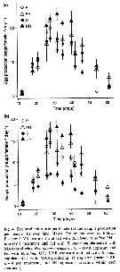 Issued from : S. Hylander, J.C. Grenvald & T. Kiørboe in Functional Eclogy, 2014, 28. [p.154, Fig.4]. Egg and nauplli production per female over time (days) function of UVR and diets. Issued from : S. Hylander, J.C. Grenvald & T. Kiørboe in Functional Eclogy, 2014, 28. [p.154, Fig.4]. Egg and nauplli production per female over time (days) function of UVR and diets.
Nota:
After Hylander & al. (2014) the life cycle from hatched egg to death lasted for ± 60 days at salinity of 27 and 18°C temperature. Copepods are known to accumulate sunscreens (so-called mycosporine-like amino acids, MAAs) and antioxydant carotenoids to mitigate negative effects of ultraviolet radiation (UVR). Cohots are followed and assessed how fitness was affected by UVR exposure and a diet rich in UVR-protective sunscreens. Copepods respond to UVR by changing the resource allocation to different fitness components resulting in reduced somatic growth, egg quality and nauplii production. Availability of sunscreens in the food source (MAAs) enables copepods to maintain high or even an elevated fitness when exposed to UVR. This illustrates that fitness coasts of UVR are diet dependent and may be considerable if UVR sunscreens are not available in the food source. Concentrations of other kinds of UVR-protective compounds such as carotenoids, are generally lower in marine than those in freshwater copepods, which suggest that predation is intense on pigmented specimens in the ocean, because the water's transparency and predation pressures are different. |
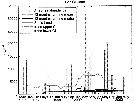 Issued from : E. Camatti, M. Pansera & A. Bergamasco inWater, 2019, 11, 1200. [p.8, Fig.4]. Issued from : E. Camatti, M. Pansera & A. Bergamasco inWater, 2019, 11, 1200. [p.8, Fig.4].
Time series of monthly A. tonsa abundance (bars) along with a 12-month running mean and median and Sen"s trend line at the San Giuliano station (Lagoon of Venice, Italy) during 1997-2002. |
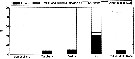 Issued from : E. Camatti, M. Pansera & A. Bergamasco inWater, 2019, 11, 1200. [p.7, Fig.3]. Issued from : E. Camatti, M. Pansera & A. Bergamasco inWater, 2019, 11, 1200. [p.7, Fig.3].
Relative abundance, station by station, of A. tonsa with respect to the other Acartia species and the remaining zooplanktonj during the 1997-2002 period in the Lagoon of Venice (Italy)
See Fig.: Study area.. |
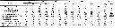 Issued from : E. Camatti, M. Pansera & A. Bergamasco inWater, 2019, 11, 1200. [p.9, Table 2]. Issued from : E. Camatti, M. Pansera & A. Bergamasco inWater, 2019, 11, 1200. [p.9, Table 2].
Average (Avg) and standard deviation (SD) values of the hydro-chemical data and biological concentration (phytoplankton), A. tonsa, and main mesozooplankton groups at the seven stations for the 2003-2004 period in the Lagoon of Venice (Italy).
See stations in the chart , fig.1.
Nota; Spatial distribution of A. tonsa was found to be significantly associated with temperature, phytoplankton, particulate organic carbon (POC), chlorophyll a, and counter gradient of salinity, confirming that A. tonsa in an opportunistic tolerant species. |
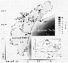 Issued from : E. Camatti, M. Pansera & A. Bergamasco inWater, 2019, 11, 1200. [p.3, Fig.1]. Issued from : E. Camatti, M. Pansera & A. Bergamasco inWater, 2019, 11, 1200. [p.3, Fig.1].
Study area (Lagoon of Venice, Italy) and location of sampling stations during 1975-1980 (grey triangles, including Lido), 1997-2002 (black circles), 2003-2004 (grey squares), and 2014-2017 (black triangles, including San Giuliano, Marghera, Fusina, and Lido.
Nota: During the decade before the first record of A. tonsa in Lagoon, the mesozooplankton community was composed of more 40 taxa. Among them, copepods were represented by 24 species and Acartia clausi being the most abundant taxon in every habitat following by A. margalefi and Paracartia latisetosa, more than 80% of the overall community.
Acartia tonsa is recently introduced in the Mediterranean Sea (Gaudy & Vinas, 1985), and only after 1985 was the presence confirmed in several Italian waters such as in a lagoon of the Po River Delta (Farabegoli & al., 1989), in the Lagoon of Lesina (Quarta & al., 1992), and in the Lagoon of Venice (Comaschi & Cavalloni, 1995).
A. tonsa was found to be the dominant species in th lagoon, while the previously dominant species of Acartiidae, Paracartia latisetosa almost disappeared, and A. margalefi not completely excluded in 2014-2017. |
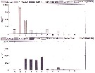 Issued from : E. Camatti, M. Pansera & A. Bergamasco in Water, 2019, 11. [p.10, Fig.5]. Issued from : E. Camatti, M. Pansera & A. Bergamasco in Water, 2019, 11. [p.10, Fig.5].
Monthly abundance of A. tonsa with respect other Acartia species remaining zooplankton at costal station 1M (top panel) and at lagoon (bottom panel) for the 2003-2004 period. (See Fig.1) |
 Issued from : R.C. Subbraju & K. Krishnamurphy in mar. Biol., 1972, 14. [p.28, Table 4] Issued from : R.C. Subbraju & K. Krishnamurphy in mar. Biol., 1972, 14. [p.28, Table 4]
Number of generations and developmental period recorded in A. clausi and A. tonsa at various localities. |
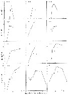 Issued from : U. Berggreen, B. Hansen & T. Kiørboe in Mar. Biol., 1988, 99. [p.344, Fig.1]. Acartia tonsa: Clearance in different developmental stages relative to equivalent spherical diameter of food algal species. Composition of developmental stages (dominating stage in bold types) at start of each experiment shown on each graph. Approximately one developmental stage will be passed during incubation, except for mature individuals. Issued from : U. Berggreen, B. Hansen & T. Kiørboe in Mar. Biol., 1988, 99. [p.344, Fig.1]. Acartia tonsa: Clearance in different developmental stages relative to equivalent spherical diameter of food algal species. Composition of developmental stages (dominating stage in bold types) at start of each experiment shown on each graph. Approximately one developmental stage will be passed during incubation, except for mature individuals.
+ Nannochloris maculata; * Pavlova lutherii; filled circle Isochrisis galbana; white square Dunaliella bioculata; open triangle Rhodomonas baltica; open circle with point Amphidinium carterae; filled triangle Thalasiosira fluviatilis; black square Scripsiella faroensis; open circle Gymnodinium splendens; x Coccinodiscus granii.
Nota: Clearance rate on different sizes of spheriocally shaped algae were determinated in uni-algal experiments for all developmental stages (NII through adult of A. tonsa, and used to construct food size spectra.
Nota: Food size spectra of Acartia tonsa were based on uni-algal experiments. It may be questioned to what extent these spectra are representative of food-selection in the field where a range of algal species/sizes are simultaneously available. Bartram (1981) and Vanderploeg & al. (1984) and both found that size-selection were invariant over a wide range of composition and concentration of natural seston and cultivated phytoplankton. For other authors, the size spectrum in suspension feeding copepods may be quite variable and modified ''taste'' ( Huntley & al., 1986), quality (Paffenhöfer & Van Sant, 1985; Ayukai, 1987), and species and size distribution (Poulet, 1973, 1974; Huntley, 1982) of food particles available as well as the 'feeding prehistory' of the copepod (Donaghay & Small, 1979; Price & Paffenhöfer, 1984 a, b) . Thus, there is evidence that particle selection in copepods (although probably variable between species) is not determined solely by particle size (suggested by Frost, 1972, 1977) but may be modified by the composition of available food (and the characters probably omnivorous or/and carnivorous). However, the maximum clearance rate is probably defined mainly by particle size (from origin vegetal or animal). The lower size limit for particle capture in Acartia tonsa is to 2 to 4 µm and fairly constant during development. Similar or higher minimum particle sizes have been found in other species (i.e. 3 µm in Pseudodiaptomus marinus nauplii and copepodites (Uye & Kasahara, 1983; 4 to 11 µm in Calanus pacificus nauplii and copepodites (Fernandez, 1979), 1 to 4 µm in Acartia tonsa and Paracalanus parvus females (Bartam, 1981), and 3 to 4 µm in Diaptomus silicis females (Vanderploeg & al., 1984). In all cases efficiency of particule capture was very low near the lower end of the food size spectra.
The size of planktonic bacteria and bactivorous flagellates is <1µm and 3 to 7 µm, respectively (Fenchel, 1982). RThus neither copepod nauplii not older stages constitute a particularly efficient link between the ''microbia loop'' and the classical food chain.
All developmental stages of suspension feeding copepods are apparently adapted to feed on particles ± 5 to 10 µm. |
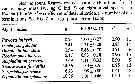 Issued from : U. Berggreen, B. Hansen & T. Kiørboe in Mar. Biol., 1988, 99. [p.343, Table 3]. Issued from : U. Berggreen, B. Hansen & T. Kiørboe in Mar. Biol., 1988, 99. [p.343, Table 3].
Regressions of clearance vs body mass on eight algal species. |
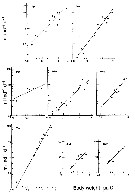 Issued from : U. Berggreen, B. Hansen & T. Kiørboe in Mar. Biol., 1988, 99. [p.345, Fig.2]. Issued from : U. Berggreen, B. Hansen & T. Kiørboe in Mar. Biol., 1988, 99. [p.345, Fig.2].
Clearance vs body mass on eight different algal species.
For each developmental stage (size) only algal species well within food size spectrum are included.
Parameters of regression analyses are given in Table 3 (p.343). |
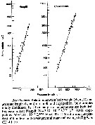 Issued from : U. Berggreen, B. Hansen & T. Kiørboe in Mar. Biol., 1988, 99. [p.346, Fig.3]. Relation between body weight and prosome length in nauplii and copepodites. Issued from : U. Berggreen, B. Hansen & T. Kiørboe in Mar. Biol., 1988, 99. [p.346, Fig.3]. Relation between body weight and prosome length in nauplii and copepodites. |
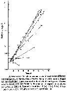 Issued from : U. Berggreen, B. Hansen & T. Kiørboe in Mar. Biol., 1988, 99. [p.346, Fig.4]. Issued from : U. Berggreen, B. Hansen & T. Kiørboe in Mar. Biol., 1988, 99. [p.346, Fig.4].
Weight increment over time at seven different concentrations of Rhodimonas baltica.
See Table 2 and 4. |
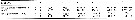 Issued from : U. Berggreen, B. Hansen & T. Kiørboe in Mar. Biol., 1988, 99. [p.343, Table 2].Rhodomonas baltica Growths experiments. Issued from : U. Berggreen, B. Hansen & T. Kiørboe in Mar. Biol., 1988, 99. [p.343, Table 2].Rhodomonas baltica Growths experiments. |
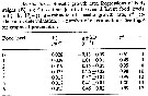 Issued from : U. Berggreen, B. Hansen & T. Kiørboe in Mar. Biol., 1988, 99. [p.346, Table 4]. Issued from : U. Berggreen, B. Hansen & T. Kiørboe in Mar. Biol., 1988, 99. [p.346, Table 4].
Specific growth rate. Regressions of body weight vs time at seven different food levels. |
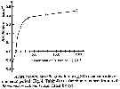 Issued from : U. Berggreen, B. Hansen & T. Kiørboe in Mar. Biol., 1988, 99. [p.346, Fig.5]. Issued from : U. Berggreen, B. Hansen & T. Kiørboe in Mar. Biol., 1988, 99. [p.346, Fig.5].
Specific growth rate over entire developmental periopd as a function of concentration of Rhodomonas baltica. |
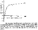 Issued from : U. Berggreen, B. Hansen & T. Kiørboe in Mar. Biol., 1988, 99. [p.349, Figs. 11]. Specific growth rate integrated over entire experimental period vs concentration ofv Rhodomonas naltica compared to specific egg-production rates claculed from Kiørboe & al. (1985). Issued from : U. Berggreen, B. Hansen & T. Kiørboe in Mar. Biol., 1988, 99. [p.349, Figs. 11]. Specific growth rate integrated over entire experimental period vs concentration ofv Rhodomonas naltica compared to specific egg-production rates claculed from Kiørboe & al. (1985). |
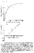 Issued from : U. Berggreen, B. Hansen & T. Kiørboe in Mar. Biol., 1988, 99. [p.348, Fig.9]. Issued from : U. Berggreen, B. Hansen & T. Kiørboe in Mar. Biol., 1988, 99. [p.348, Fig.9].
a: Specific ingestion integrated over entire experimental period relative to concentration of R. baltica
b: Specific growth vs specific ingestion rate both integrated over entire experimental period. |
 Issued from : U. Berggreen, B. Hansen & T. Kiørboe in Mar. Biol., 1988, 99. [p.342, Table 1]. Issued from : U. Berggreen, B. Hansen & T. Kiørboe in Mar. Biol., 1988, 99. [p.342, Table 1].
Linear dimension (length x breadth), equivalent mean spherical diameter (ESD) and carbon and nitrogen content of cultured phytoplankton used in experiments.
ESD was measured by a Coulter Counter except for Gymnodinium spendens and Coccinodiscus granii where it was calculated from linear dimensions.
C:N = weight ratio of carbon to nitrogen. n = number of determinations of N- and C-content. Mean ±SD. |
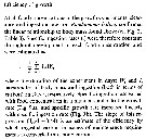 Issued from : U. Berggreen, B. Hansen & T. Kiørboe in Mar. Biol., 1988, 99. [p.347]. Issued from : U. Berggreen, B. Hansen & T. Kiørboe in Mar. Biol., 1988, 99. [p.347].
Algorithm of the specific ingestion rates. |
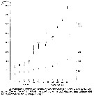 Issued from : J.G. Støttrup, K. Richardson, E. Kirkegaard & N.J. Pihl in Aquaculture, 1986, 52. [p.93, Fig.3]. Issued from : J.G. Støttrup, K. Richardson, E. Kirkegaard & N.J. Pihl in Aquaculture, 1986, 52. [p.93, Fig.3].
Acartia tonsa cephalothorax lengths and widths reared in the laboratory from the Danish Institute for Fisheries and Marine Research.
Cultivated continuously by Rhodomonas baltica (Cryptophyte), maintened at 16-18°C, as the copepods in the tanks. |
 Issued from : J.G. Støttrup, K. Richardson, E. Kirkegaard & N.J. Pihl in Aquaculture, 1986, 52. [p.92, Table 1]. Issued from : J.G. Støttrup, K. Richardson, E. Kirkegaard & N.J. Pihl in Aquaculture, 1986, 52. [p.92, Table 1].
Total number of eggs produced and feeding concentrations registered during February 1985 for the two tanks in laboratory.
The generation time, defined as the duration from egg to the point in time when 50% of the females are fertilized, is approximately 20 days at 18°C. Mortality is almost constant at 5%/day |
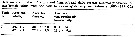 Issued from : J.G. Støttrup, K. Richardson, E. Kirkegaard & N.J. Pihl in Aquaculture, 1986, 52. [p.92, Table 2]. Issued from : J.G. Støttrup, K. Richardson, E. Kirkegaard & N.J. Pihl in Aquaculture, 1986, 52. [p.92, Table 2].
Number of adults and females/l and daily average minimal production of eggs/female taken from tanks in laboratoty during January and February 1985.
Eggs are harvestede daily and, on average, ca. 25 eggs are collected per female per day. |
 Issued from : G. Drillet, P.M. Jepsen, J.K. Højgaard, N.O.G. Jørgensen & B. W. Hansen in Aquaculture, 2008, 279. [p.50, Table 1]. Acartia tonsa strains: Issued from : G. Drillet, P.M. Jepsen, J.K. Højgaard, N.O.G. Jørgensen & B. W. Hansen in Aquaculture, 2008, 279. [p.50, Table 1]. Acartia tonsa strains:
Mean duration (days - d-1 ±S.E. (n = 4 replicates) of the different development stages from different geographic sites (DIFRES: strain originated from cosatal site in Øresund, Denmark; Kiel, Germany, Turkey Point, Florida, USA and Mobile Bay, Alabama, USA).
The experimental target is to identify a strains which produce preys with a highly valuable chemical composition.
Experimental cultivation in bottles were incubated at 17°C, Sal. 34 ppt, oxygen (4.5-9.4 mg. -1) and pH (8.0-8.3) measured daily throughout the experiments, and copepods reared with algal concentrations of Rhodomonas salina.
The four strains showed distinct patterns of development. For all strains, except Kiel, the main peak in nauplii was observed within 2 days of incubation (though a few eggs from Denmark hatced a biot later), while eggs of Kiel strain developed into nauplii later and peaked at 8 days.
Copepodite stages appeared after 7 to 8 days for all strains.
Adult stages were observed after 11, 10, 15 and 10 days in the different strains (Denmark-Alabama), respectively.
Average time required for hatching (time to switch from egg to naupliar stage) was higher for the Kiel eggs than for the three other strains and ranged from 1.05±0.02 days to 2.78±0.45 days for Alabama and Kiel, respectively.
The time required to switch to the copepodite stage was shortest in the Alabama strain (7.9 days), followed by Denmark strain (8.4 days). These two strains differed significantly from both Kiel and Florida.
Copepodites of the Alabama strain were the first to reach adulthood (after 13.7 days), followed by Denmark (after 14.6 days), while copepodites from Kiel and Florida reached adulthood after 17.5 days and 18.6 days, respectively
The DIFRES and Alabama strains had both shorter generation time (period for development from egg to adulthood).. |
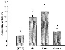 Issued from : G. Drillet, P.M. Jepsen, J.K. Højgaard, N.O.G. Jørgensen & B. W. Hansen in Aquaculture, 2008, 279. [p.50, Fig.2]. Acartia tonsa strains: Issued from : G. Drillet, P.M. Jepsen, J.K. Højgaard, N.O.G. Jørgensen & B. W. Hansen in Aquaculture, 2008, 279. [p.50, Fig.2]. Acartia tonsa strains:
Mortality rate for Denmark (DIFRES), Kiel, Florida and Alabama strains (mortality d-1).
Bars and whiskers are for the mean ±SE. There are no statistical differences between means annotated with the same letter (SNK, p < 0.05).
See algorithm used for the instantaneous rates of mortality claculated.
The average daily mortality of the strains varied from 4.01 to 5.67 % (Denmark and Alabama) and from 11.6 to 13.8 % (Kiel and Florida).
The mortality rates of the Denmark and Alabama were statistically different from both the Kiel and the Florida strains but not from one another (SNK, p <0.05). |
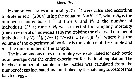 Issued from : G. Drillet, P.M. Jepsen, J.K. Højgaard, N.O.G. Jørgensen & B. W. Hansen in Aquaculture, 2008, 279. [p.48]. Instantaneous rates of mortality calculated for the different strains ofAcartia tonsa. Algorithm according to Breteler & al. (2004). Issued from : G. Drillet, P.M. Jepsen, J.K. Højgaard, N.O.G. Jørgensen & B. W. Hansen in Aquaculture, 2008, 279. [p.48]. Instantaneous rates of mortality calculated for the different strains ofAcartia tonsa. Algorithm according to Breteler & al. (2004). |
 Issued from : G. Drillet, P.M. Jepsen, J.K. Højgaard, N.O.G. Jørgensen & B. W. Hansen in Aquaculture, 2008, 279. [p.50, Table 2]. Acartia tonsa: mean sex ratios calculated for all strains. Issued from : G. Drillet, P.M. Jepsen, J.K. Højgaard, N.O.G. Jørgensen & B. W. Hansen in Aquaculture, 2008, 279. [p.50, Table 2]. Acartia tonsa: mean sex ratios calculated for all strains.
In all strains, the sex ratio was in favour of females, making up 53.9 to 69.3 %.
In comparisons between strains, the sex ratio for the Florida was found to be significantly different from Denmark and Kiel sex ratios, but not from Alabama (SNK, p < 0.05, n = 27).
Within strains, the differences between genders (male: female) were significant for Denmark, Florida and Alabama, but not for the Kiel population. |
 Issued from : G. Drillet, P.M. Jepsen, J.K. Højgaard, N.O.G. Jørgensen & B. W. Hansen in Aquaculture, 2008, 279. [p.50, Table 3]. Acartia tonsa strains. Issued from : G. Drillet, P.M. Jepsen, J.K. Højgaard, N.O.G. Jørgensen & B. W. Hansen in Aquaculture, 2008, 279. [p.50, Table 3]. Acartia tonsa strains.
Daily mean egg production and accumulation of daily egg production.
Nota: Significant differences in egg production were observed among the four strains.
Individual females produced between 0 and 78 eggs day-1. The daily mean egg production over three days for each strain varied from 37.2 to 50.5 eggs.
The Denmark strain had higher average egg production than the Kiel and Florida strains (SNK, p < 0.05), and the Alabama strain had higher production than the Kiel strain (SNK, p < 0.05). |
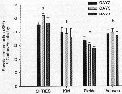 Issued from : G. Drillet, P.M. Jepsen, J.K. Højgaard, N.O.G. Jørgensen & B. W. Hansen in Aquaculture, 2008, 279. [p.51, Fig.3]. Acartia tonsa strains. Issued from : G. Drillet, P.M. Jepsen, J.K. Højgaard, N.O.G. Jørgensen & B. W. Hansen in Aquaculture, 2008, 279. [p.51, Fig.3]. Acartia tonsa strains.
Specific egg production (SEP) of the Denmark (DIFRES), Kiel, Florida and Alabama strains. Means ± SE. (n = 8 to 13). There are no statistical differences between means annotated with the sale letter (Dunn's, p < 0.05).
The average specific egg production (SEP), calculated as production of carbon (C) relative to C content for each female over 3 days, ranged from 17.2 to 55.8 % C female day-1.
However, on particular days some females had a SEP as hugh as 60.9 % of their body weight day-1.
Adult cephalothorax length ranged from 850 to 900 µm, and mean egg diameter was 83.8b ±0.4 µm, and 82.7 ±0.2 µm, 77.9 ±0.3 µm, and 78.8 ±0.5 µm for Denmark (DIFRES), Kiel, Florida, and Alabama eggs, respectively (Drillet & al., 2008).
The average SEP over 3 days ranged from 30.3 to 51.8 %. All strains showed significantly different SEP values, except Alabama vs. Kiel. |
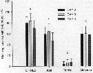 Issued from : G. Drillet, P.M. Jepsen, J.K. Højgaard, N.O.G. Jørgensen & B. W. Hansen in Aquaculture, 2008, 279. [p.51, Fig.4]. Acartia tonsa strains. Issued from : G. Drillet, P.M. Jepsen, J.K. Højgaard, N.O.G. Jørgensen & B. W. Hansen in Aquaculture, 2008, 279. [p.51, Fig.4]. Acartia tonsa strains.
Hatching success within 48 h of eggs.
Means ±SE (n = 8 to 13) shown.
There are no statistical differences between means annotated with the same letter (Dunn's, p < 0.05).
hatching success, defined as mean percentage of hatched eggs within 48 h, ranged from 47.3 to 83.8 % for eggs of the Denmark (DIFRES), Kiel and Alabama strains, but were significantly lower in the Florida strain, ranging from 4.1 to 7.2 %. |
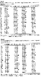 Issued from : G. Drillet, P.M. Jepsen, J.K. Højgaard, N.O.G. Jørgensen & B. W. Hansen in Aquaculture, 2008, 279. [p.51, Table 4, 5]. Acartia tonsa strains. Issued from : G. Drillet, P.M. Jepsen, J.K. Højgaard, N.O.G. Jørgensen & B. W. Hansen in Aquaculture, 2008, 279. [p.51, Table 4, 5]. Acartia tonsa strains.
Table 4 : Relative quantities of free amino acid 5FFA) in eggs (% of total FAA±SE) and number of replicates (n) used for analysis.
Eggs of all strains were characterized by a high fraction of proline (Pro) 34-43 %, though, the Floridian eggs showed a lower proportion of proline than the two Baltic strains. The floridian eggs had a higher content of Asn than the other 3 strains and higher content of taurine (Tau), a non protein amino acid, than the Baltic strains (7.7 and 11.4 %, respectively (p < 0.05).
The Denmark (DIFRES) strain had a lower content of histamine (His) than the other strains (4.8 % vs 7.9 % or more). Finally, these eggs of the danish strain had a higher proportion of Ile than all the other strains (1.9 % vs. 1.2 or less).
No significant differences were observed between strains in egg content of free amino acid (FAA) relative to dry weight. All strains contained approximaterly 6-8 % FAA relative to dry weight (DW).
Table 5 : Relative quantities of free amino acid in females (% of FAA ±SE) and number of replicates (n) used for analysis.
In the females, there was no single dominant FAA. Instead, a few FAA made up between 8 % and 15 % of all FAA.
Common FAA were Histamine, Taurine, Arginine, Alamine and Proline, and to a lesser extent, Leucine and Lysine.
Kiel and Alabama females had a significantly higher proportion of Taurine than the other groups (P < 0.05).
Kiel females presented a lower proportion of tyrosine (Tyr) and Valine (Val) than the other strains.
Significant differences in the fatty acid ratio of docosahexaenoic acid (DHA)/ eicosapentaenoic acid (EPA) were observed between eggs but not between adults of different strains. Mean ratios of DHA to EPA in the eggs were 0.82, 1.37, 1.34 and 1.48 for Florida, Denmark, Kiel and Alabvama strains. The differences were significant between eggs of all strains, but not between Denmark and Kiel eggs. In the adults, the DHA/EPA ratio was higher and ranged from 2.1 to 2.45, but not significant differences were observed (SNK, p < 0.05). |
 Issued from : G. Drillet, E. Goetze, P.M. Jepsen, J.K. Højgaard & B.W. Hansen in Aquaculture, 2008, 280. [p.111, Fig.2]. Issued from : G. Drillet, E. Goetze, P.M. Jepsen, J.K. Højgaard & B.W. Hansen in Aquaculture, 2008, 280. [p.111, Fig.2].
Genetic analysis of strains Acartia tonsa from four sites: DIFRES (Øresund, Denmark, 56°N, 123°E), Kiel Bight , Germany (SW Baltic Sea, 54°N, 10°E), Turquey point (Florida, USA, 29°55'N, 84°30'W), Mobile Bay (Alabama, USA, 30°N, 87°W). |
 Issued from : G. Drillet, E. Goetze, P.M. Jepsen, J.K. Højgaard & B.W. Hansen in Aquaculture, 2008, 280. [p.112, Table 1]. Issued from : G. Drillet, E. Goetze, P.M. Jepsen, J.K. Højgaard & B.W. Hansen in Aquaculture, 2008, 280. [p.112, Table 1].
Genetic differentiation between experimental strains.
Nota: The mitochondrial COI alignment was 658 bp in length, and contained 140 variable sites, 136 of which were parsimony informative. Across all strains, and including data from 31 individuals, a total of 8 halotypes were observed. The average number of nucleotide differences between haplotypes within each strain did not exceed 0.16%, and within strain nucleotide diversity (py) ranged from 0.00036-0.00163.
The rRNA alignment was 129 bp in length, following truncation of the alignment to include only those nucleotide sites shared with A. tonsa sequences from Caudill & Bucklin (2004). The alignment included 39 variable sites, 29 of which were parsimony informative, and no indels were present in the alignment. A total of four 16S rRNA haplotypes were observed among all strains. A maximum of 0.03% in the average number of nucleotide differences between haplotypes within each strain was observed at this gene.
The four experimental strains derived from three highly distinct mitochondrial clades within the nominal species A. tonsa (see in Fig.2 A, B). The Denmark (DIFRES) and Kiel strains were genetically indistinguishable at both COI and 16S rRNA gene loci, indicating that they originate from the same lineage of A. tonsa within the Baltic Sea.
The Turkey point (Florida) and Mobile Bay (Alabama) strains were highly divergent from one another, as well as from the Denmark/Kiel European lineage. As estimated by Kimura 2-parameter distance measures, these three lineages were divergent by 14-17.45% at COI and 10.95-16.49% at 16S rRNA. The average number of nucleotide differences between lineages ranged from 12.51-14.90% at COI and 10.08-14.90% at 165 rRNA.
Phylogenetic results from mtCOI and mt 16S rRNA analyses were in agreement regarding the position of the experimental strains within the phylogeny of A. tonsa, as expected given linkage of these gene loci. Caudill & Bucklin (2004, Fig.1) descrived four divergent 16S rRNA mitochondrial clades, which they identified as containing 'A', 'B', 'C', and 'D' haplotypes. The authors will continue to refer to these clades by their letter designations.
Analysis of 165 rRNA sequences found 4 reciprocally-monophyletic clades, which had bootstrap support values of 84-100% in both parsimony and likelihood analyses (see Fig.2, A). The DIFRES/Kiel strain was found to be closely related to the 'A' clade, while the Mobile Bay (Alabama) and Turkey Point (Florida) strains were members of the 'B' and 'C' clades, respectively. (see fig.2A).
Analysis of mtCOI data identified 3 reciprocally-monophyletic clades, each of which had between 78 and 100% bootstrap support in parsimony and likelihood analyses (see Fig.2, B).Data from the experimental strains of the authors was analyzed in conjunction with A. tonsa COI sequences available in GenBank (Bucklin & al., unpub; Durbin & al., 2008). Current sampling at COI has recovered only 3 on 4 known mitochondrial clades, with the Mobile Bay AL and RI, FL, AL (see in Fig.2,B) clade corresponding to clade 'B', DIFRES/Kiel and RI/Europa corresponding to clade 'A', and Turkey Pt, FL representing clade 'C' (see in Fig.2, B). Although parsimony analysis recovered 150 equal-length trees, these trees differed only in the relative positions of haplotypes within the Mobile Bay, RI, FL, AL clade 'B' and were stable with regard to placement of haplotypes across clades and the positions of haplotypes within clades 'A' and 'C'. One observation of note is that one of the DIFRES/KIEL strain hapoltypes was 100% identical to a haplotype sampled in Rhode Island (USA).
The broad-scale phylogeographic structure of A. tonsa is currently unclear. However, this nominal species contains at least 4 deep mitochondrial clades, of which, clade 'A' appears to have colonised European brackish waters. The DIFRES/Kiel experimental strain, isolated from waters in the southern Baltic and in the Øresund was found to contain a COI genetically identical to a haplotype present in Rhode Island (USA) which may indicate an East coast US source for the invasive populations in Europe. A. tonsa was first reported in European waters in the Caen Canal (France), in 1927 (Rémy, 1927)., followed by subsequent reports extending the range of the species to estuaries throughout Europe, including the Baltic, Mediterranean and Black Sea. |
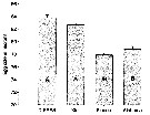 Issued from : G. Drillet, E. Goetze, P.M. Jepsen, J.K. Højgaard & B.W. Hansen in Aquaculture, 2008, 280. [p.113, Fig.3]. Issued from : G. Drillet, E. Goetze, P.M. Jepsen, J.K. Højgaard & B.W. Hansen in Aquaculture, 2008, 280. [p.113, Fig.3].
Egg size of Acartia tonsa cultures from four geographic areas, raised in a common garden experiment at 17°C.
Bars labeled A and B have significantly different mean values (Kruskal-Wallis on Ranks, Dunn's method, p <0.001).Nota: Egg diameter was 83.8 ±0.4 µm, 82.7 ±0.2 µm, 77.09 ±0.3 µm, and 78.8 ±0.5 µm for Denmark (DIFRES), Kiel, Florida and Albanama eggs, respectively (mean ±S.E.). There were significant differences in egg size between the Gulf of Mexico and Baltic strains, but not within these two groups of strains. |
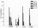 Issued from : G. Drillet, E. Goetze, P.M. Jepsen, J.K. Højgaard & B.W. Hansen in Aquaculture, 2008, 280. [p.113, Fig.4]. Issued from : G. Drillet, E. Goetze, P.M. Jepsen, J.K. Højgaard & B.W. Hansen in Aquaculture, 2008, 280. [p.113, Fig.4].
Hatching success at 17°C of eggs from the four Acartia tonsa strains produced at 17°C and stored subsequently at 5.4 ±0.7 °C for a range of storage durations.
For each strain, bar color indicates increasing periods of storage (inset legend). Figures represent the mean ±S.E.
Nota: Eggs from Florida and Alabama rapidly lost their viability over time, and showed increased mortality after 30 days of cold storage.
After 60 days of cold storage, no survival was observed in eggs from either strain. Florida and Alabama hatching successes were significantly lower than the DIFRES (Denmark) strain from day 20 onwards. Eggs from DIFRES were more resistant to cold storage, and 5 ±1.2% hatched after 150 days. Hatching success of DIFRES eggs was significantly different from the other three strains on all days except Alabama on day 10
Eggs from the Kiel population showed the most surprising trend in hatching pattern during the cold-storage period. At day 10, the lowest hatching success was observed for this strain, but subsequently increased with the length of the cold storage period from 7 % hatching after 10 days to 35 ±2% hatching after 100 days and 30 ±4% hatching after 150 days of cold storage
The hatching success of Kiel eggs was significantly different from all strains on all days with the exception, of Alabama and Florida on day 30. |
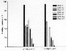 Issued from : G. Drillet, E. Goetze, P.M. Jepsen, J.K. Højgaard & B.W. Hansen in Aquaculture, 2008, 280. [p.113, Fig.5]. Issued from : G. Drillet, E. Goetze, P.M. Jepsen, J.K. Højgaard & B.W. Hansen in Aquaculture, 2008, 280. [p.113, Fig.5].
Hatching success at 17°C and 25°C of eggs from Denmark (DIFRES) strains of Acartia tonsa produced at 17°C or 25°C and stored subsequently at 5.4 ±0.7 °C for a range storage durations.
For each strain, bar color indicates increasing periods of storage (inset legend). Figures represent the mean ±S.E.
Parental rearing temperature was observed to be an important factor influencing egg survivorship during cold storage.
Eggs produced by DIFRES females kept at 25°C showed a constant decrease in hatching success over the storage period while eggs produced at 17°C seemed to have a more stable hatching success, around 40%, between day 10 and day 60. After 100 days of cold storage, the hatching success of eggs produced at 17°C and 25°C had declined to 47% and 12%, respectively. After 150 days, the hatching capacities of eggs produced at both temperatures were low, but some survival was still observed. From day 30 onwards, eggs produced at 25°C showed lower survival the eggs raised at 17°C.
The Baltic Sea strains appear to have produced eggs with two different resting strategies, quiescence and delayed hatching, under these common garden conditions, despite a lack of genetic differentiation at two mitochondrial loci between these laboratory strains.
The DIFRES strain produced eggs that had maximal hatching success at initiation of the experiment and declined with age, as would be expected for subitaneous eggs. The Kiel strain, however, produced eggs with relatively low hatching success at the biginning of the experiment (31%), with a minimum in hatching at 10 days (7%) followed by increased hatching success later in the experiment (up to 35% after 100 days). Eggs cold stored for 150 days had high levels of viability, and showed a 30% final hatching success. Freshly spawned eggs from the Kiel strain also showed a significantly prolonged hatching period in a related stage-development experiment (Drillet & al., 2008), which they considered unusual for A. tonsa subitaneous eggs at this temperature. Based on these results the authors conclude that a fraction of the Kiel eggs were entering a delayed-hatching state, rather than simply being in a state of quiescence. It is, however, currently unclear which environmental conditions acted as cue (s) for induction of this type of dormancy in eggs of this starin, as eggs from previous generations were hatching in a pattern similar to that presently observed in the DIFRES strain (pers. obs.). The light regime was intentionnaly chosen to follow the spring/early summer rhythm, because A. tonsa is known to exhibit winter diapause in the egg stage (Castro-Longoria, 2001); hence, it seems unlikely that light conditions were acting as cues for the partial dormancy switch. One possibility is that A. tonsa resting eggs production may be affected by the presence of copepod metabolites in the relatively dense culture, as been demonstrated for Eurytemora affinis (Ban & Minoda, 1994).
Given the genetic similarity between the two nBaltic strains, it may also be possible to deliberately induce dormant eggs in the DITRES strain under the correct environmental conditions.
Egg survivorship in quiescent eggs of the DIFRES strain may be impacted by oxygen concentration during cold storage.
One important aspect, not studied, is the effect of long-term egg storage (months) on the biochemical composition of eggs, which could also affect naupliar quality (Drillet & al., 2006 a, b). Such an effect was not observed during short-term storage of subitaneous eggs from the Florida strain (Sedlacek & Marcus, unpubl.). Changes in biochemical composition of eggs and nauplii may influence mortality rate, impact their palatability and nutritional value to fish. |
 Issued from : J.N. Putland & R.L. Iverson in Mar. Ecol. Progr. Ser., 2007, 340. [p.173. Abstract part.] Issued from : J.N. Putland & R.L. Iverson in Mar. Ecol. Progr. Ser., 2007, 340. [p.173. Abstract part.]
Acartia tonsa were studied within various salinity regimes in Apalachicola Bay (Florida) throughout a 2 years period.
The percent of phytoplankton productivity ingested by animal ranged from 0 to 24% (median 0.4%). The diet was mixed. On average, 53% of the diet was composed of phytoplankton.
Per capita total ingestion rate averaged 1.1 ±1.3 (±SD) µg C adult-1 day -1 during winter, peaked to about 6 µg C adult-1 day-1 during summer, and averaged 2.2 ±1.8 µg C adult-1 day-1 during summer.
A. tonsa ingested the equivalent of 38 ±48% and 120 ± 93% of its body carbon during winter and summer, respectively.
During summer, per capita total ingestion rate increased below 20 psu.
Average egg production rate was lower during winter (13 ±215 eggs female-1 day-1) than during summer (28 ±24 eggs female-1 day -1. During summer the egg production rate peaked between about 4 and 10 psu. During winter and summer, egg production efficiency peaked between about 8 and 14 psu.
Salinity tolerance and biochemical composition of phytoplankton ingested may have influenced the egg production efficiency. Phytoplankton allocated more carbvon to protein and lipid synthesis in lower salinity water. The areal extent of lower (<20 psu) salinity water decreases in the bay during periods when river discharge is low. Therefore, upstream water diversion during summer can be expected to reduce the areal extent of lower (<20 psu) salinity waters where ingestion rate, egg production efficeincy, and egg production rate of A. tonsa are greatest and where A. tonsa is an important prey for Anchoa mitchilli.
Nota (CR): psu: conductivity in µ Sienens cm-1.
fresh water between 500 to 1000; brackish: about 10,000 µs (salt: ± 6.5 /1000).
µS cm-1 x 0.36 = Chlorinity; x0.58 = NaCl; x 0.65 = salt total (mg l-1. |
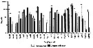 Issued from : C. de O. Dias, Carvalho P.F. de, A.C.T Bonecker & S.L.C. Bonecker in Ocean Coastal Management, 2018, 161. [p.198, Fig.11]. Issued from : C. de O. Dias, Carvalho P.F. de, A.C.T Bonecker & S.L.C. Bonecker in Ocean Coastal Management, 2018, 161. [p.198, Fig.11].
Variation of seasonal mean (± SD) density (Log ind.m3. of Temora turbinatain Guanabara Bay (22°50'S, 43°10'W).
Zooplankton collected from January 2012 to December 2013 in front of Icaral beach during the flood time, by horizontal subsurface hauls (1 m depth), net of 200 µm mesh aperture.
For the authors, the study shows that the poor conditions in the Guanabara Bay are aggravated during periods of rainfall, and that the increase of micriobiological indictors affectes the biodiversity of organisms in the mesoplanktonic community.
The copepods Temora turbinata and Acartia tonsa presented the highest densities throughout the study perod. The dominance in the Bay has changed considerably in recent years; untill two decades ago Temora turbinata and Acartia tonsa were not even registered in the Bay, probably explained by introduction through ship ballast water at ports on the Brazilian coast. These two species have been reported as dominant species which shows their great capacity for adaptation and reproduction in a short time period.
Acartia tonsa has been reported on Guanabara Bay since 1990s, while T. turbinata in 2000 (Guenther & al., 2012; Bonecker & al., 2012)
In the study area, Acartia lilljeborgi previously was reported as the most abundant species in the Bay. The success of A. tonsa can be attributed in eutrophic environments given the wide availability of food and the omnivory of this species; during certain periods, phytoplankton and microzooplankton are scarce, so suspended pareticles and detritus become the main food for the filter-feeding consumers. Detritus also supplements the algae-based diet of A.tonsa (Menéndez & al., 2011).
For the authors, the restructuring of the local community may be related to the constant degradation of the environment, particularly in the inner areas of the bay, reflecting in the entire ecosystem (Gomes, 2007). |
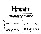 Issued from : C. de O. Dias, Carvalho P.F. de, A.C.T Bonecker & S.L.C. Bonecker in Ocean Coastal Management, 2018, 161. [p.192 Figs.2, 3]. Issued from : C. de O. Dias, Carvalho P.F. de, A.C.T Bonecker & S.L.C. Bonecker in Ocean Coastal Management, 2018, 161. [p.192 Figs.2, 3].
Variation s of values of precipitation (mm) and seasonal mean (± SD) of temperature and salinity during 2012-2013 years at Guanabara Bay (Brazil). |
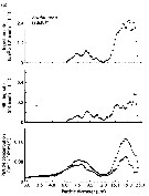 Issued from : C.B. Miller in Biological Oceanography 2004/2005, Blackwell Publishing. [p.139, Fig.7.6]. Issued from : C.B. Miller in Biological Oceanography 2004/2005, Blackwell Publishing. [p.139, Fig.7.6].
Exemple of selection by particle-feeding copepods from Chesapeake Bay. (a) The particle spectra before (dark circles) and after (open circles a day of feeding by female Acartia tonsa, which avoided eating particles near 12 µm equivalent spherical diameter. (After Richman, Heinle & Huff, 1977). |
Issued from : C.B. Miller in Biological Oceanography 2004/2005, Blackwell Publishing. [p.157, Table 7.1]. After Heinle, 1966.
Acartia tonsa dominant zooplankters in coastal waters from Chesapeake Bay (USA). Data characterize the season of peak production. Mostly taken from Landry (1978): 80 mgC m-2 day-1.
Miller underlines the difficulties of the production estimations for single species,
and virtually none for whole systems, but we would like to know how much food the oceans produces for animals we harvest like herring, anchovy, cod, and pollack. See Huntley & Lopez, 1992: model); Kleppel, Davis & Carter, 1996; Huntley, 1996; Hirst & Sheader, 1997; Hirst & Lampitt, 1998; Vidal, 1980. |
 Issued from : S. Ban, C. Burns, J. Castel, Y. Chaudron & al. in Mar. Ecol. Prog. Ser., 1997, 157. [p.289, Table 1]. Issued from : S. Ban, C. Burns, J. Castel, Y. Chaudron & al. in Mar. Ecol. Prog. Ser., 1997, 157. [p.289, Table 1].
Synopsis of feeding/reproduction experiments. A total of 17 diatom and 16 copepod species, representative of a variety of worldwide temperate and subarctic environments (E: estuarine, C: coastal ocean), were screened.
Data for fecundity and hatching success are average values measured at the start and end of the inciubations in a minimum of 3 replicate batches, showing the variation in time of the effects of diatoms on copepod reproduction.
Level of significance of the diatom effect between treatments and controls (e.g. non-diatom diets) in categories I to III was p < 0.01. No.. rank (for comparison with Table 2, p.290).
For the signification of the categories I to IV (fecundity vs. Hatching success vs. Duration of experiment days-1): See Calanus finmarchicus.
List of the 12 marine or estuarine species studied (fresh water excluded. CR): Acartia clausi, A. grani, A. steueri, A. tonsa, Calanus finmarchicus, C. helgolandicus, C. pacificus, Centropages hamatus, C. typicus, Eurytemora affinis, Temora longicornis, T. stylifera. |
 Issued from : S. Ban, C. Burns, J. Castel, Y. Chaudron & al. in Mar. Ecol. Prog. Ser., 1997, 157. [p.290, Table 2]. Issued from : S. Ban, C. Burns, J. Castel, Y. Chaudron & al. in Mar. Ecol. Prog. Ser., 1997, 157. [p.290, Table 2].
Combinations of copepod and non-diatom diets in controls in concentrations ranging from 104 to 105 cells ml-1. Data for fecundity and hatching success are average values measured at the start and end of incubation in a minimum of 3 replicate batches.
UF: unidentified flagellates.
In Category I. |
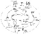 Issued from : E. Camatti, A. Comaschi, J. Coppola, L. Milani, M. Minocci & G. Socal in Biol. Mar. Medit., 2006, 13 (1). [p.51, Fig.5]. Issued from : E. Camatti, A. Comaschi, J. Coppola, L. Milani, M. Minocci & G. Socal in Biol. Mar. Medit., 2006, 13 (1). [p.51, Fig.5].
Schematic representation of mezozooplankton species succession over an annual cycle in the lagoon of Venice (data from 1975 to 2004).
The species in the external ellipse are perennant taxa. |
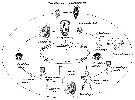 Issued from : E. Camatti, A. Comaschi, J. Coppola, L. Milani, M. Minocci & G. Socal in Biol. Mar. Medit., 2006, 13 (1). [p.50, Fig.4]. Issued from : E. Camatti, A. Comaschi, J. Coppola, L. Milani, M. Minocci & G. Socal in Biol. Mar. Medit., 2006, 13 (1). [p.50, Fig.4].
Schematic representation of microzooplankton species succession over an annual cycle in the lagoon of Venice (data from 2003 to 2004).
The species in the external ellipse are perennant taxa.
See Fig. 5 copepod composition. |
| | | | Loc: | | | Falkland Is., Ushuaia, Beagle Channel, Magellan Strait, Magallanes region, Patagonia, Peninsula Valdés, Mar del Plata, Argentina (Bahia Blanca estuary), Uruguay (Laguna de Rocha, continental shelf), off Rio de la Plata, Brazil (paranagua Bay,Vitoria Bay, Guanabara Bay, Mucuri estuary, Saco de Mangueira, Lagoa dos Patos Cananeia Lagoon, Curuça estuary, Ajuruteua Beach, Taperaçu estuary, Caeté Estuary, Amazon estuary, off Amazon), Guyana (Kourou), off Angola, Congo, G. of Guinea (Liberia, Ghana), Morocco-Mauritania, Caribbean Colombia, Cariaco Basin, Venezuela, Jamaica, Caribbean Sea (Yucatan), Chelem lagoon, Colombia (Laguna Navio Quebrado), G. of Mexico, La Habana Bay, Turkey Point, off Timbalier Island, Mississipi (off Southwest Pass), Mississipi River (plume), Jamaica, Porto-Rico, Savannah River Estuary, Florida, Bayboro Harbor, Wassaw Sound, off Bermuda, Port Aransas Channel (Texas); Miami, Patuxent River estuary, Avery Point, off Maryland, Wilmington River estuary, Newport River estuary, Patuxent River, Beaufort (Inlet, Gallants Channel), Chesapeake Bay, Hampton River, Delaware Bay, Long Island Sound, Narragansett Bay, Great Bay, New York, Long Island, off Woods Hole, Damariscotta esuary, Perch Pond, Buzzards Bay, Cap Cod, Nova Scotia, Bras d'Or Lake, Morrison's Pond, Shédiac Bay, Northumberland Strait, G. of St. Lawrence, North Sea, Baltic Sea, Gulf of Mecklenburger, Bay of Kiel, Schlei Fjord, Elbe (estuary), Dunkerque Harbour, English Channel, Southampton, Bay of Biscay (Arcachon Bay), Gironde Estuary, Bilbao estuary, Portugal (Ria de Aveiro, Mondego estuary), Medit. (Berre Lagoon, Livorno, Lake Faro, G. of Gabes, NW Adriatic Sea: Po estuary, Lagoon of Venezzia, S. Adriatic Sea (Lesina lagoon), Koper Harbour, Lebanon Basin, Marmara Sea, Black Sea, Sevastopol Bay, Azov Sea), Caspian Sea, Indian (Maldive Is.), Singapore, Indonesia-Malaysia, Caroline Is., Vancouver Is., off Washington coast, Oregon (Yaquina, off Newport), San Francisco (Bay and Estuary), Monterey Bay, Los Angeles (San Pedro Bay), San Diego (Bay), off La Jolla, W Baja California (Bahia Magdalena), G. of California (N & Centre, lagoon Agiabampo: Sonora, Coyuca lagoon: Guerrero), La Paz, W Mexico, E Australia, Pacif. S (NPFZ), Bahia Cupica (Colombia), Galapagos-Ecuador, off Peruvian coast, Chile ( N, off Concepcion, Mejillones Bay, Valparaiso, off Santiago) | | | | N: | 481 | | | | Lg.: | | | (16) F: 1,12-0,9; (36) F: 1,27-1,1; M: 1,12-0,98; (46) F: 1,5-1,3; M: 1,05; (142) F: 1,5-1,2; M: 1,1-1; (145) F: 1,4; M: 1,34; (179) F: 0,97-0,87; M: 0,8-0,77; (187) F: 1,4-1,12; M: 1,14-1,03; (188) F: 1,5-1,3; M: 1,05; (237) F: 1,25; M: 1,0; (237 as giesbrechti*) F: 1,0; (253) F: 0,98-0,821; M: 0,84-0,786 [Black Sea]; F: 1,15-1,029; M: 1-0,91 [S Adriatic Sea]; (817) F: 1,25; M: 1,09; (254) F: ±1,25; M: ±1; (861) F: 1,44-1,46; M: 1,21-1,23; (1125) F: 1,0-1,2; {F: 0,821-1,50; M: 0,77-1,34} | | | | Rem.: | côtière, ± saumâtre.
Rémy, 1927 a (p.177 & suiv.) a analysé la répartition géographique de cette espèce à partir de sa description dans la baie de Port-Jackson (Australie). Il en déduit que les localisations, notamment sur les côtes européennes, pourraient être dues à des transports par navires. Récemment Carlton & Geller (1993, p.78) et Mauchline (1998, p.505) en ont donné quelques exemples.
Zillioux & Gonzalez (1972) furent les premiers à signaler la présence d'oeufs de "durée" dans les fonds marins chez des copépodes pélagiques.
La P5 femelle peut présenter des anomalies (cf. Behrends & al., 1997).
D'après Saiz et Kiørboe (1995), l'espèce présente deux modes différents de nutrition. Lorsqu'il se nourrit de petites cellules phytoplanctoniques il crée un courant se comportant comme un 'suspension feeder', et losqu'il se nourrit à partir de proies mobiles il montre un comportement à l'atffût ('ambush feeder").
Voir aussi les remarques en anglais | | | Dernière mise à jour : 04/03/2026 | |
|
|
 Toute utilisation de ce site pour une publication sera mentionnée avec la référence suivante : Toute utilisation de ce site pour une publication sera mentionnée avec la référence suivante :
Razouls C., Desreumaux N., Kouwenberg J. et de Bovée F., 2005-2026. - Biodiversité des Copépodes planctoniques marins (morphologie, répartition géographique et données biologiques). Sorbonne Université, CNRS. Disponible sur http://copepodes.obs-banyuls.fr [Accédé le 10 juin 2026] © copyright 2005-2026 Sorbonne Université, CNRS
|
|
|
|

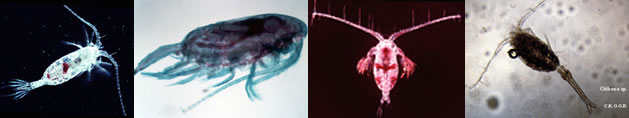


 tonsa - Planche 1 de figures morphologiques',750,500);)
 tonsa - Planche 2 de figures morphologiques',750,500);)
 tonsa - Planche 3 de figures morphologiques',750,500);)
 tonsa - Planche 4 de figures morphologiques',750,500);)
 tonsa - Planche 5 de figures morphologiques',750,500);)
 tonsa - Planche 6 de figures morphologiques',750,500);)
 tonsa - Planche 7 de figures morphologiques',750,500);)
 tonsa - Planche 8 de figures morphologiques',750,500);)
 tonsa - Planche 9 de figures morphologiques',750,500);)
 tonsa - Planche 10 de figures morphologiques',750,500);)
 tonsa - Planche 11 de figures morphologiques',750,500);)
 tonsa - Planche 13 de figures morphologiques',750,500);)
 tonsa - Planche 14 de figures morphologiques',750,500);)
 tonsa - Planche 15 de figures morphologiques',750,500);)
 tonsa - Planche 16 de figures morphologiques',750,500);)
 tonsa - Planche 17 de figures morphologiques',750,500);)
 tonsa - Planche 18 de figures morphologiques',750,500);)
 tonsa - Planche 19 de figures morphologiques',750,500);)
 tonsa - Planche 20 de figures morphologiques',750,500);)
 tonsa - Planche 21 de figures morphologiques',750,500);)
 tonsa - Planche 22 de figures morphologiques',750,500);)
 tonsa - Planche 23 de figures morphologiques',750,500);)
 tonsa - Planche 24 de figures morphologiques',750,500);)
 tonsa - Planche 25 de figures morphologiques',750,500);)
 tonsa - Planche 26 de figures morphologiques',750,500);)
 tonsa - Planche 27 de figures morphologiques',750,500);)
 tonsa - Planche 28 de figures morphologiques',750,500);)
 tonsa - Planche 29 de figures morphologiques',750,500);)
 tonsa - Planche 30 de figures morphologiques',750,500);)
 tonsa - Planche 32 de figures morphologiques',750,500);)
 tonsa - Planche 33 de figures morphologiques',750,500);)
 tonsa - Planche 34 de figures morphologiques',750,500);)
 tonsa - Planche 35 de figures morphologiques',750,500);)
 tonsa - Planche 37 de figures morphologiques',750,500);)
 tonsa - Planche 38 de figures morphologiques',750,500);)
 tonsa - Planche 39 de figures morphologiques',750,500);)

 tonsa - Carte de distribution 4',650,500);)
 tonsa - Carte de distribution 5',750,500);)
 tonsa - Carte de distribution 6',750,500);)
 tonsa - Carte de distribution 9',750,500);)
 tonsa - Carte de distribution 10',750,500);)
 tonsa - Carte de distribution 11',750,500);)
 tonsa - Carte de distribution 12',750,500);)
 tonsa - Carte de distribution 14',750,500);)
 tonsa - Carte de distribution 15',750,500);)
 tonsa - Carte de distribution 18',750,500);)
 tonsa - Carte de distribution 19',750,500);)
 tonsa - Carte de distribution 20',750,500);)
 tonsa - Carte de distribution 22',750,500);)
 tonsa - Carte de distribution 24',750,500);)
 tonsa - Carte de distribution 25',750,500);)
 tonsa - Carte de distribution 26',750,500);)
 tonsa - Carte de distribution 27',750,500);)
 tonsa - Carte de distribution 28',750,500);)
 tonsa - Carte de distribution 29',750,500);)
 tonsa - Carte de distribution 31',750,500);)
 tonsa - Carte de distribution 32',750,500);)
 tonsa - Carte de distribution 33',750,500);)
 tonsa - Carte de distribution 35',750,500);)
 tonsa - Carte de distribution 38',750,500);)
 tonsa - Carte de distribution 39',750,500);)
 tonsa - Carte de distribution 41',750,500);)
 tonsa - Carte de distribution 42',750,500);)
 tonsa - Carte de distribution 43',750,500);)
 tonsa - Carte de distribution 46',750,500);)
 tonsa - Carte de distribution 47',750,500);)
 tonsa - Carte de distribution 49',750,500);)
 tonsa - Carte de distribution 50',750,500);)
 tonsa - Carte de distribution 51',750,500);)
 tonsa - Carte de distribution 52',750,500);)
 tonsa - Carte de distribution 53',750,500);)
 tonsa - Carte de distribution 55',750,500);)
 tonsa - Carte de distribution 56',750,500);)
 tonsa - Carte de distribution 57',750,500);)
 tonsa - Carte de distribution 58',750,500);)
 tonsa - Carte de distribution 60',750,500);)
 tonsa - Carte de distribution 61',750,500);)
 tonsa - Carte de distribution 65',750,500);)
 tonsa - Carte de distribution 66',750,500);)
 tonsa - Carte de distribution 69',750,500);)
 tonsa - Carte de distribution 70',750,500);)
 tonsa - Carte de distribution 71',750,500);)
 tonsa - Carte de distribution 72',750,500);)
 tonsa - Carte de distribution 73',750,500);)
 tonsa - Carte de distribution 74',750,500);)
 tonsa - Carte de distribution 75',750,500);)
 tonsa - Carte de distribution 76',750,500);)
 tonsa - Carte de distribution 78',750,500);)
 tonsa - Carte de distribution 79',750,500);)
 tonsa - Carte de distribution 80',750,500);)
 tonsa - Carte de distribution 84',750,500);)
 tonsa - Carte de distribution 85',750,500);)
 tonsa - Planche 1 de figures morphologiques)
 tonsa - Planche 2 de figures morphologiques)
 tonsa - Planche 3 de figures morphologiques)
 tonsa - Planche 4 de figures morphologiques)
 tonsa - Planche 5 de figures morphologiques)
 tonsa - Planche 6 de figures morphologiques)
 tonsa - Planche 7 de figures morphologiques)
 tonsa - Planche 8 de figures morphologiques)
 tonsa - Planche 9 de figures morphologiques)
 tonsa - Planche 10 de figures morphologiques)
 tonsa - Planche 11 de figures morphologiques)
 tonsa - Planche 12 de figures morphologiques)
 tonsa - Planche 13 de figures morphologiques)
 tonsa - Planche 14 de figures morphologiques)
 tonsa - Planche 15 de figures morphologiques)
 tonsa - Planche 16 de figures morphologiques)
 tonsa - Planche 17 de figures morphologiques)
 tonsa - Planche 18 de figures morphologiques)
 tonsa - Planche 19 de figures morphologiques)
 tonsa - Planche 20 de figures morphologiques)
 tonsa - Planche 21 de figures morphologiques)
 tonsa - Planche 22 de figures morphologiques)
 tonsa - Planche 23 de figures morphologiques)
 tonsa - Planche 24 de figures morphologiques)
 tonsa - Planche 25 de figures morphologiques)
 tonsa - Planche 26 de figures morphologiques)
 tonsa - Planche 27 de figures morphologiques)
 tonsa - Planche 28 de figures morphologiques)
 tonsa - Planche 29 de figures morphologiques)
 tonsa - Planche 30 de figures morphologiques)
 tonsa - Planche 31 de figures morphologiques)
 tonsa - Planche 32 de figures morphologiques)
 tonsa - Planche 33 de figures morphologiques)
 tonsa - Planche 34 de figures morphologiques)
 tonsa - Planche 35 de figures morphologiques)
 tonsa - Planche 36 de figures morphologiques)
 tonsa - Planche 37 de figures morphologiques)
 tonsa - Planche 38 de figures morphologiques)
 tonsa - Planche 39 de figures morphologiques)
 tonsa - Carte de distribution 4)
 tonsa - Carte de distribution 5)
 tonsa - Carte de distribution 6)
 tonsa - Carte de distribution 7)
 tonsa - Carte de distribution 8)
 tonsa - Carte de distribution 9)
 tonsa - Carte de distribution 10)
 tonsa - Carte de distribution 11)
 tonsa - Carte de distribution 12)
 tonsa - Carte de distribution 13)
 tonsa - Carte de distribution 14)
 tonsa - Carte de distribution 15)
 tonsa - Carte de distribution 16)
 tonsa - Carte de distribution 17)
 tonsa - Carte de distribution 18)
 tonsa - Carte de distribution 19)
 tonsa - Carte de distribution 20)
 tonsa - Carte de distribution 21)
 tonsa - Carte de distribution 22)
 tonsa - Carte de distribution 23)
 tonsa - Carte de distribution 24)
 tonsa - Carte de distribution 25)
 tonsa - Carte de distribution 26)
 tonsa - Carte de distribution 27)
 tonsa - Carte de distribution 28)
 tonsa - Carte de distribution 29)
 tonsa - Carte de distribution 30)
 tonsa - Carte de distribution 31)
 tonsa - Carte de distribution 32)
 tonsa - Carte de distribution 33)
 tonsa - Carte de distribution 34)
 tonsa - Carte de distribution 35)
 tonsa - Carte de distribution 36)
 tonsa - Carte de distribution 37)
 tonsa - Carte de distribution 38)
 tonsa - Carte de distribution 39)
 tonsa - Carte de distribution 40)
 tonsa - Carte de distribution 41)
 tonsa - Carte de distribution 42)
 tonsa - Carte de distribution 43)
 tonsa - Carte de distribution 44)
 tonsa - Carte de distribution 45)
 tonsa - Carte de distribution 46)
 tonsa - Carte de distribution 47)
 tonsa - Carte de distribution 48)
 tonsa - Carte de distribution 49)
 tonsa - Carte de distribution 50)
 tonsa - Carte de distribution 51)
 tonsa - Carte de distribution 52)
 tonsa - Carte de distribution 53)
 tonsa - Carte de distribution 54)
 tonsa - Carte de distribution 55)
 tonsa - Carte de distribution 56)
 tonsa - Carte de distribution 57)
 tonsa - Carte de distribution 58)
 tonsa - Carte de distribution 59)
 tonsa - Carte de distribution 60)
 tonsa - Carte de distribution 61)
 tonsa - Carte de distribution 62)
 tonsa - Carte de distribution 63)
 tonsa - Carte de distribution 64)
 tonsa - Carte de distribution 65)
 tonsa - Carte de distribution 66)
 tonsa - Carte de distribution 67)
 tonsa - Carte de distribution 68)
 tonsa - Carte de distribution 69)
 tonsa - Carte de distribution 70)
 tonsa - Carte de distribution 71)
 tonsa - Carte de distribution 72)
 tonsa - Carte de distribution 73)
 tonsa - Carte de distribution 74)
 tonsa - Carte de distribution 75)
 tonsa - Carte de distribution 76)
 tonsa - Carte de distribution 77)
 tonsa - Carte de distribution 78)
 tonsa - Carte de distribution 79)
 tonsa - Carte de distribution 80)
 tonsa - Carte de distribution 81)
 tonsa - Carte de distribution 82)
 tonsa - Carte de distribution 83)
 tonsa - Carte de distribution 84)
 tonsa - Carte de distribution 85)