|
|
 |
Fiche d'espèce de Copépode |
|
|
Cyclopoida ( Ordre ) |
|
|
|
Oncaeidae ( Famille ) |
|
|
|
Triconia ( Genre ) |
|
|
| |
Triconia conifera (Giesbrecht, 1891) (F,M) | |
| | | | | | | Syn.: | Oncäa conifera Giesbrecht, 1891; 1892 (p.591, 603, 774, figs.F,M);
no O. conifera : Sars, 1900 (p.113);
no Oncaea conifera var. III Giesbrecht, 1902 (p.41, Pl.13, figs.7-11);
no O. conifera : Tanaka, 1960 (p.66, figs.F,M); B.D. Lee, 1966;
no Oncaea conifera : Farran, 1936 a (p.127, figs.F: forms b & c);
no O. conifera : Moulton, 1973 (p.147 & suiv.:'minus');
Oncaea conifera : Vanhöffen, 1897 a (p.281); Thompson & Scott, 1903 (p.239, 285); Norman, 1903 b (p.141); Esterly, 1905 (p.216, figs.F); Pearson, 1906 (p.35); Carl, 1907 (p.17); Farran, 1908 b (p.92); A. Scott, 1909 (p.241, Rem.); Wolfenden, 1911 (p.362); Pesta, 1912 a (p.57, fig.F); 1913 (p.33); Lysholm, 1913 (p.7); Brady, 1918 (p.34, figs.F); Pesta, 1920 (p.651, fig.); Willey, 1920 a (p.24); Lysholm & Nordgaard, 1921 (p.29); Farran, 1926 (p.296); 1929 (p.210, 285); Rose, 1929 (p.58); Wilson, 1932 a (p.350, figs.F,M); Rose, 1933 a (p.298, figs.F,M); Hardy & Gunther, 1935 (1936) (p.190, Rem.); Farran, 1936 a (p.127, figs.F, Rem.: forme a); Mori, 1937 (1964) (p.120, figs.F); Jespersen, 1940 (p.91); Dakin & Colefax, 1940 (p.116, figs.F); Lysholm & al., 1945 (p.43); Sewell, 1947 (p.259, Rem.F, p.259-260: Rem.); Davis, 1949 (p.76); Vervoort, 1951 (p.150, Rem.); Krishnaswamy, 1953 (p.68, Rem.); Østvedt, 1955 (p.15: Table 3, p.79); Vervoort, 1957 (p.146, Rem.); Chiba & al., 1957 (p.310); 1957 a (p.12); Minoda, 1958 (p.253, Table 1, 2, abundance); Marques, 1958 a (p.135, figs.F); Fagetti, 1962 (p.42); Björnberg, 1963 (p.80, Rem.); Kasturirangan, 1963 (p.78, figs.F,M); Anraku & Azeta, 1965 (p.13, Table 2, fish predator); Shmeleva, 1965 b (p.1350, lengths-volume-weight relation); Saraswathy, 1966 (1967) (p.102); Owre & Foyo, 1967 (p.111, figs.F,M); Ramirez, 1969 (p.89, figs.F,M, Rem.); Kovalev, 1970 (p.91, Tableau 1, 2, fig., egg production); Corral Estrada, 1970 (p.220, Rem); Minoda, 1971 (p.44); Shih & al., 1971 (p.56, 156, 215); Björnberg, 1972 (p.93); Bradford, 1971 b (p.28); Razouls, 1972 (p.95, Annexe: p.114, figs.F); Bradford, 1972 (part., p.50, figs.F,M); Chatton & M.O. Soyer, 1973 (p.27, fig.2, parasite); Moulton, 1973 (p.141, Rem.: 4 groupes, variétés); Chen & al., 1974 (p.41, figs.F,M, p.75: Rem, Group "a" from Farran, 1936); Marques, 1975 (p.50, figs.F); Ferrari, 1975 (p.218, figs.F,M, Rem.); Palet, 1975 (p.660); Boxshall, 1977 a (p.138, figs.F,M, Rem..); Dawson & Knatz, 1980 (p.9, 10, figs.F,M); Björnberg & al., 1981 (p.667, figs.F,M); Dessier, 1983 (p.89, Tableau 1, 2, Rem., %); Malt, 1983 (p.457, figs.F, Rem.); Malt, 1983 a (p.6, figs.F,M, Rem.: varieties); Herman A.W., 1984 (p.131, Rem.: p.133); Kim & al., 1993 (p.271); Seguin & al., 1993 (p.23); Heron & Bradford-Grieve, 1995 (p.17, figs.F,M); ? Mazzochi & al., 1995 (p.229, figs.F,M, Rem.); Menshenina & Melnikov, 1995 (p.129); Ohtsuka & al., 1996 a (p.91); Chihara & Murano, 1997 (p.979, Pl.225: F,M); Boxshall, 1998 (p.225); Noda & al., 1998 (p.55, Table 3, occurrence); Lapernat, 1999 (p.35, Rem.); Avancini & al., 2006 (p.133, Pl. 101, figs.F,M, Rem.);
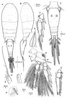
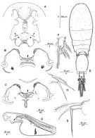
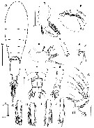
Ref. compl.: Mrazek, 1902 (p.517, 524); Cleve, 1904 a (p.193); Damas & Koefoed, 1907 (p.395, tab.II); Rose, 1925 (p.152); Wilson, 1942 a (p.198); Sewell, 1948 (p.346, 461, 487, 515); C.B. Wilson, 1950 (p.271); Ganapati & Shanthakumari, 1962 (p.10, 16); V.N. Greze, 1963 a (tabl.2); Duran, 1963 (p.25); Giron-Reguer, 1963 (p.58); Grice, 1963 a (p.496); Gaudy, 1963 (p.32, Rem.); Unterüberbacher, 1964 (p.34); De Decker & Mombeck, 1964 (p.13); Mazza, 1966 (p.73); Pavlova, 1966 (p.45); Neto & Paiva, 1966 (p.31, Table III, annual cycle); Furuhashi, 1966 a (p.295, vertical distribution vs mixing Oyashio/Kuroshio region, Table 9); Ehrhardt, 1967 (p.743, 887, geographic distribution, Rem.); De Decker, 1968 (p.45); Evans, 1968 (p.14); Delalo, 1968 (p.139); Kovalev, 1970 (p.91, Tableau 1, 2, fig., egg production); Salah, 1971 (p.320); Deevey, 1971 (p.224); Bainbridge, 1972 (p.61, Appendix Table I: vertical distribution vs day/night, Table II: %); Binet & al., 1972 (p.71); Apostolopoulou, 1972 (p.329, 379); Björnberg, 1973 (p.363, 388); Corral Estrada Pereiro Muñoz, 1974 (tab.I); Vives & al., 1975 (p.56, 57, tab.II, III, IV, XII); Vives, 1976 (p.104); Peterson & Miller, 1976 (p.14, Table 1, 3, abundance vs interannual variations); 1977 (p.717, Table 1, seasonal occurrence); Zalkina, 1977 (p.339, tab.1); Deevey & Brooks, 1977 (tab.2); Dessier, 1979 (p.207); Pipe & Coombs, 1980 (p.223, figs. 1, 2, 4, table 1, vertical distribution); Herman & Mitchell, 1981 (p.739, Table 2, length-volume); Herman & Sameoto, 1981 (p.228, Table 1, 2, abundance); Haury & Wiebe, 1982 (p.915, horizontal micro-distribution); Vives, 1982 (p.295); Rudyakov, 1982 (p.208, Table 2); Kovalev & Shmeleva, 1982 (p.85); Scotto di Carlo & Ianora, 1983 (p.150); Scotto di Carlo & al., 1984 (p.1041); Sameoto, 1984 (p.213, Table 1); 1984 a (p.767, vertical migration); Tremblay Anderson, 1984 (p.7); Sazhina, 1985 a (p.491, tab.3); Moraitou-Apostolopoulou, 1985 (p.303, occurrence/abundance in E Mediterranean Sea, Rem.: p.310); Longhurst, 1985 (tab.2); Jansa, 1985 (p.108, Tabl.I, II, III, IV); M. Lefèvre, 1986 (p.33, 40); Zmijewska, 1987 (tab.2a); Lozano Soldevilla & al., 1988 (p.61); Dessier, 1988 (tabl.1); Böttger-Schnack & al., 1989 (p.1089); Hirakawa & al., 1990 (tab.3); Yoo, 1991 (tab.1); Scotto di Carlo & al., 1991 (p.270); Lampitt & al., 1993 (p.689, faecal pellets v.s. ingestion); Landry & al., 1994 (p.55, abundance, grazing); Kouwenberg, 1994 (tab.1); Böttger-Schnack, 1994 (p.277); 1995 (p.92); Gonzalez & al., 1994 (p.331); Shih & Young, 1995 (p.76); Hajderi, 1995 (p.542); Kotani & al., 1996 (tab.2); Böttger-Schnack, 1996 (p.1086); 1997 (p.409); Suarez-Morales & Gasca, 1997 (p.1525); Park & Choi, 1997 (Appendix); Go & al., 1998 (p.475, Table 1, feeding behavior); Krsinic, 1998 (p.1051); Hure & Krsinic, 1998 (p.83, 104); Alvarez-Cadena & al., 1998 (t.1,2,3,4); Suarez-Morales & Gasca, 1998 a (p.112); Siokou-Frangou, 1999 (p.479); Dolganova & al., 1999 (p.13, tab.1); Lavaniegos & Gonzalez-Navarro, 1999 (p.239, Appx.1); Bragina, 1999 (p.196); Razouls & al., 2000 (p.343, tab. 5, Appendix); Seridji & Hafferssas, 2000 (tab.1); Escribano & Hidalgo, 2000 (p.283, tab.2); Lopez-Salgado & al., 2000 (tab.1); Kosobokova & Hirche, 2000 (p.2029, tab.2);El-Sherif & Aboul Ezz, 2000 (p.61, Table 3: occurrence); Hidalgo & Escribano, 2001 (p.159, tab.2); Hidalgo & Escribano, 2001 (p.157, fig.4); d'Elbée, 2001 (tabl.1); Li & al., 2001 (p.894, tab.1); Zerouali & Melhaoui, 2002 (p.91, Tableau I); Conway & al., 2003 (p.220, figs.F,M, Rem.); Lo & al., 2004 (p.468, tab.2); Lan & al., 2004 (p.332, tab.1); Lo & al., 2004 (p.89, tab.1); Kazmi, 2004 (p.231); Prusova & Smith, 2005 (p.76); Obuid Allah & al., 2005 (p.123, occurrence % vs metal contamination); Lopez-Ibarra & Palomares-Garcia, 2006 (p.63, Tabl. 1, seasonal abundance vs El-Niño); Dias & Araujo, 2006 (p.87, Rem., chart); Mageed, 2006 (p.171, Table 4); Escribano, 2006 (p.20, Table 1); Deibel & Daly; 2007 (p.271, Table 4, Rem.: Arctic polynyas); Hwang & al., 2007 (p.25); Castro & al., 2007 (486, fig.3, Table 1, 2, 3); Jitlang & al., 2008 (p.65, Table 1); Rakhesh & al., 2008 (p.154, Table 5: abundance vs stations); Morales-Ramirez & Suarez-Morales, 2008 (p.525); Tseng L.-C. & al., 2008 (p.153, fig.5, Table 2, occurrence vs geographic distribution, indicator species); Lopez Ibarra, 2008 (p.1, Table 1, fig.11: abundance); Ayon & al., 2008 (p.238, Table 4: Peruvian samples); C.-Y. Lee & al., 2009 (p.151, Tab.2); Galbraith, 2009 (pers. comm.); Chiba & al., 2009 (p.1846, Table 1, occurrence vs temperature change); Lan Y.-C. & al., 2009 (p.1, Table 2, % vs hydrogaphic conditions); Licandro & Icardi, 2009 (p.17, Table 4); Escribano & al., 2009 (p.1083, Table 1, figs.6, 10); Brugnano & al., 2010 (p.312, Table 3, fig.8); Hafferssas & Seridji, 2010 (p.353, Table 3); Lidvanov & al., 2010 (p.356, Table 3); Drira & al., 2010 (p.145, Tanl.2); Medellin-Mora & Navas S., 2010 (p.265, Tab. 2); Hsiao S.H. & al., 2011 (p.475, Appendix I); Hsiao & al., 2011 (p.317, Table 2, indicator of seasonal change); Zhang G.-T. & Wong, 2011 (p.277, fig.7, indicator, as Oncaea conifer); Kâ & Hwang, 2011 (p.155, Table 3: occurrence %); Maiphae & Sa-ardrit, 2011 (p.641, Table 2, 3, Rem.); Selifonova, 2011 a (p.77, Table 1, alien species in Black Sea); Tseng L.-C. & al., 2011 (p.47, Table 2, occurrences vs mesh sizes); Tutasi & al., 2011 (p.791, Table 2, 3, abundance distribution vs La Niña event); Glushko & Lidvanov, 2012 (p.138, Tableau 1, 3); Brugnano & al., 2012 (p.207, Table 2); Rekik & al., 2012 (p.336, Table 1, abundabce); Jang M.-C & al., 2012 (p.37, Table 3: as Oncaea conifer, abundance and seasonal distribution); Tseng & al., 2013 (p.507, seasonal abundance); Rakhesh & al., 2013 (p.7, Table 1, abundance vs stations); Jagadeesan & al., 2013 (p.27, Table 3, seasonal variation); Anjusha & al., 2013 (p.40, Table 3, abundance & feeding behavior); Lidvanov & al., 2013 (p.290, Table 2, % composition); Zaafa & al., 2014 (p.67, Table I, occurrence); Nakajima & al., 2015 (p.19, Table 3: abundance); Palomares-Garcia & al., 2018 (p.178, Table 1: occurrence) | | | | Ref.: | | | Böttger-Schnack, 1999 (p.43, 53, Redescr.F,M, figs.F,M, Rem.); Böttger-Schnack & al., 2004 (p.1130, tab.1, Rem.); Vives & Shmeleva, 2010 (p.341, figs.F,M, Rem.); Wi & al., 2010 (p.679, Redescr., figs.F,M, Rem.); 2011 (p.601, Rem.: variations); Böttger-Schnack & Machida, 2011 (p.111, Table 1, 2, fig.2, 3 DNA sequences, phylogeny); Wi & al., 2012 (p.857, Rem.); Böttger-Schnack & Schnack, 2015 (p.10: Rem.) | 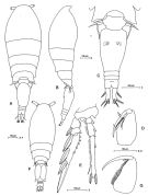 Issued from: M.G. Mazzocchi, G. Zagami, A. Ianora, L. Guglielmo & J. Hure in Atlas of Marine Zooplankton Straits of Magellan. Copepods. L. Guglielmo & A. Ianora (Eds.), 1995. [p.231, Fig.3.43.1]. As Oncaea conifera. With doubt. Female: A, habitus (dorsal); B, idem (lateral right side); C, urosome (dorsal); D, Mxp; E, P4. Nota: Proportional lengths of prosome and urosome 64:36. Proportional lengths of urosomites and furca 16:48:5:5:10:16 = 100. Caudal rami almost 3 times longer than wide. Male: F, habitus (dorsal); G, Mxp. Nota: Proportional lengths of prosome and urosome 66:34. Proportional lengths of urosomites and furca 8:51:14:2:2:11:12 = 100. Genital somite with postero-lateral flap on ventral surface; flap bearing denticulated margin on ventral side and minute, hyaline denticules on both ventral and dorsal surfaces.
|
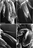 Issued from: M.G. Mazzocchi, G. Zagami, A. Ianora, L. Guglielmo & J. Hure in Atlas of Marine Zooplankton Straits of Magellan. Copepods. L. Guglielmo & A. Ianora (Eds.), 1995. [p.235, Fig.3.43.5]. As Oncaea conifera. With doubt. Male (SEM preparation): A, Urosome and P4 (ventral); B, extremity of last segment of P4 endopod; C, P5; D, Mxp. Bars: A 0.050 mm; B-D 0.010 mm.
|
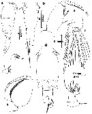
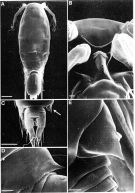 Issued from: M.G. Mazzocchi, G. Zagami, A. Ianora, L. Guglielmo & J. Hure in Atlas of Marine Zooplankton Straits of Magellan. Copepods. L. Guglielmo & A. Ianora (Eds.), 1995. [p.234, Fig.3.43.4]. As Oncaea conifera. With doubt. Male (SEM preparation): A, habitus (dorsal); B, forehead (ventral); C, urosome (dorsal); D, postero-lateral flap on genital somite (ventral, arrow in C); E, same flap (dorsal). Bars: A 0.100 mm; B, D, E 0.010 mm; C 0.050 mm.
|
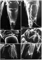 Issued from: M.G. Mazzocchi, G. Zagami, A. Ianora, L. Guglielmo & J. Hure in Atlas of Marine Zooplankton Straits of Magellan. Copepods. L. Guglielmo & A. Ianora (Eds.), 1995. [p.233, Fig.3.43.3]. As . With doubt.
Female (SEM preparation): A, urosome (dorsal); B, urosome (dorsal) with attached ovigerous sac; C, P5; D, Mxp; E, P4; F, detail of distal endopodal segment of P4.
Bars: A, B, C, D 0.050 mm; E, 0.100 mm; F, 0.010 mm.
|
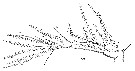
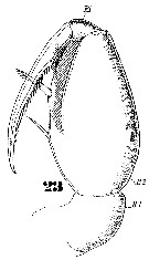
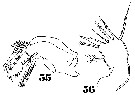
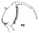
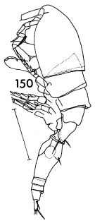 issued from : F.C. Ramirez in Contr. Inst. Biol. mar., Buenos Aires, 1969, 98. [p.98, Lam. XVIII, fig.150 ]. As Oncaea conifera. Female (from off Mar del Plata): 150, habitus (lateral left side). Scale bar in mm: 0.3.
|
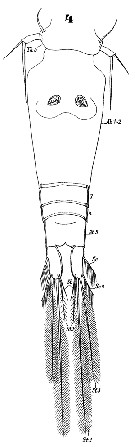
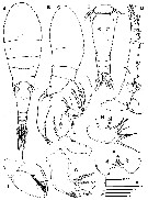
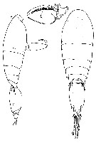
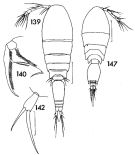 issued from : F.C. Ramirez in Contr. Inst. Biol. mar., Buenos Aires, 1969, 98. [p.86, Lam. XVII, figs.139, 140, 142, 147]. As Oncaea conifera. Female (from off Mar del Plata): 139, habitus (dorsal); 140, Mxp; 142, P5. Male: 147, habitus (dorsal). Scale bars in mm: 0.2 (139); 0.4 (142); 0.2 (147).
|
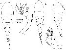
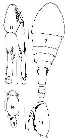
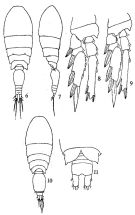 issued from : Q.-c Chen & S.-z. Zhang & C.-s. Zhu in Studia Marina Sinica, 1974, 9. [Pl.6, Figs.6-11]. As Oncaea conifera. Female (from China Seas): 6, habitus (dorsal); 7, idem (lateral right side); 8, P3; 9, P4. Male: 10, habitus (dorsal); 11, posterior portion of abdomen).
|
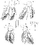
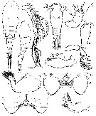
 issued from : R. Böttger-Schnack in Mitt. hamb. zool. Mus. Inst., 1999, 96 [p.54, Fig.6]. Female (from Red Sea): A, habitus (dorsal); B, idem (lateral left side), appendages omitted; C, urosome (dorsal); D, A1 (6th segment, small spinule arrowed); E, endopod of P2 (anterior, setae omitted); F, exopod of P3 (anterior, setae omitted); G, P4 (posterior), raised secretory pore arrowed, other surface ornamentation not figured [g, inner portion of basis, showing variation of tip]; H, P6; I, Md (dorsal blade); J, spine of P1 exopod 3 (showing subapical tubular exyrnsion, arrowed). Nota: Proportional lengths (%) of urosomites and caudal rami 11.4:50.6:6.3:6.6:12.7:12.3.
|
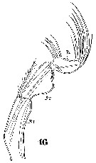
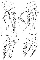
 issued from : R. Böttger-Schnack in Mitt. hamb. zool. Mus. Inst., 1999, 96 [p.56, Fig.7]. Female: A, rostral area and labrum, anterior (arrows indicating position of lateral concavity); B, labrum, anterior (straight margin between lobes arrowed); D, P5 (dorsal). Male (from Red Sea): E, habitus (dorsal); F, caudal ramus; G, Mxp (lateral, secretory pore on syncoxa arrowed); H, P5. Nota: Proportional lengths (%) of urosomites and caudal rami 10.2:52.6:3.2:3.1:3.2:11.6:9.0.
|
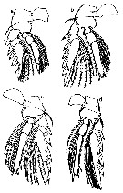
 issued from : G.A. Boxshall in Bull. Br. Mus. nat. Hist. (Zool.), 1977, 31 (3). [p.139, Fig.19]. As Oncaea conifera. Female (from 18°N, 25°W): a, habitus 'stocky form' (lateral); b, urosome (ventral); c, P4 (posterior); d, Mxp (anterior); e, Md (anterior); f, Mx1 (anterior). Male: g, urosome (ventral); h, Mxp (posterior; i, A2 (anterior).
|
 issued from : G.A. Boxshall in Bull. Br. Mus. nat. Hist. (Zool.), 1977, 31 (3). [p.140, Fig.20, a-c]. Female: habitus 'stocky form' (dorsal); b, habitus 'long form' c, habitus 'bumped form' (dorsal); d, A2 'stocky form' (anterior); e, A2 'bumped form' (anterior).
|
 issued from : Z. Zheng, S. Li, S.J. Li & B. Chen in Marine planktonic copepods in Chinese waters. Shanghai Sc. Techn. Press, 1982 [p.99, Fig.58]. As Oncaea conifera. Female: a-b, habitus (dorsal and lateral, respectively); c, Mxp; d, P3; e, P4. Scale bars in mm.
|
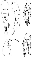
 issued from : J.M. Bradford in Mem. N. Z. Oceonogr. Inst., 1972, 54. [p.51, Fig.14, (7-10, 13-14]. As Oncaea conifera. Female (from Kaikoura, New Zealand): 7, habitus (dorsal); 8, Mxp; 9, P2 (endopod segment 3); 10, P4 (endopod segment 3). Male: 13, Mxp; 14, urosome (dorsal). Scale bars: 0.1 mm.
|
 Issued from : W. Giesbrecht in Systematik und Faunistik der Pelagischen Copepoden des Golfes von Neapel und der angrenzenden Meeres-Abschnitte. Fauna Flora Golf. Neapel, 1892, 19 , Atlas von 54 Tafeln. [Taf.47, Fig.4]. As Oncäa conifera. Female: 4, urosome (dorsal).
|
 Issued from : W. Giesbrecht in Systematik und Faunistik der Pelagischen Copepoden des Golfes von Neapel und der angrenzenden Meeres-Abschnitte. Fauna Flora Golf. Neapel, 1892, 19 , Atlas von 54 Tafeln. [Taf.47, Fig.21]. As Oncäa conifera. Female: 21, A1 (from over).
|
 Issued from : W. Giesbrecht in Systematik und Faunistik der Pelagischen Copepoden des Golfes von Neapel und der angrenzenden Meeres-Abschnitte. Fauna Flora Golf. Neapel, 1892, 19 , Atlas von 54 Tafeln. [Taf.47, Fig.23]. As Oncäa conifera. Female: 23, Mxp.
|
 Issued from : W. Giesbrecht in Systematik und Faunistik der Pelagischen Copepoden des Golfes von Neapel und der angrenzenden Meeres-Abschnitte. Fauna Flora Golf. Neapel, 1892, 19 , Atlas von 54 Tafeln. [Taf.47, Figs.55, 56]. As Oncäa conifera. Female: 55, Md; 56, Mx1.
|
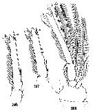 Issued from : W. Giesbrecht in Systematik und Faunistik der Pelagischen Copepoden des Golfes von Neapel und der angrenzenden Meeres-Abschnitte. Fauna Flora Golf. Neapel, 1892, 19 , Atlas von 54 Tafeln. [Taf.47, Figs.36, 37, 38]. As Oncäa conifera. Female: 36, endopod of P3; 37, endopod of P2; 38, endopod of P4.
|
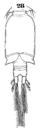 Issued from : W. Giesbrecht in Systematik und Faunistik der Pelagischen Copepoden des Golfes von Neapel und der angrenzenden Meeres-Abschnitte. Fauna Flora Golf. Neapel, 1892, 19 , Atlas von 54 Tafeln. [Taf.47, Fig.28]. As Oncäa conifera. Male: 28, urosome (ventral).
|
 Issued from : W. Giesbrecht in Systematik und Faunistik der Pelagischen Copepoden des Golfes von Neapel und der angrenzenden Meeres-Abschnitte. Fauna Flora Golf. Neapel, 1892, 19 , Atlas von 54 Tafeln. [Taf.47, Fig.42]. As Oncäa conifera. Male: 42, Mxp.
|
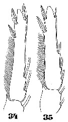 Issued from : W. Giesbrecht in Systematik und Faunistik der Pelagischen Copepoden des Golfes von Neapel und der angrenzenden Meeres-Abschnitte. Fauna Flora Golf. Neapel, 1892, 19 , Atlas von 54 Tafeln. [Taf.47, Figs.34, 35]. As Oncäa conifera. Male: 34, endopod of P3; 35, endopod of P2.
|
 Issued from : W. Giesbrecht in Systematik und Faunistik der Pelagischen Copepoden des Golfes von Neapel und der angrenzenden Meeres-Abschnitte. Fauna Flora Golf. Neapel, 1892, 19 , Atlas von 54 Tafeln. [Taf.47, Fig.16]. As Oncäa conifera. Female: 16, Mxp.
|
 issued from : J.H. Wi, R. Böttger-Schnack & H.Y. Soh in J. Crustacean Biol., 2010, 30 (4). [p.680, Fig.5]. Female (from 34°05.97'N, 129°47.32'E): A-B, habitus (dorsal and lateral, respectively); C, urosome (dorsal); D, A1; E, A2; F, labrum (posterior); G, Md; H, Mx1; I, Mxp. Scale bars in micrometers.
|
 issued from : J.H. Wi, R. Böttger-Schnack & H.Y. Soh in J. Crustacean Biol., 2010, 30 (4). [p.681, Fig.6]. Female: P1 to P4 respectively (anterior vews). Scale bars in micrometers.
|
 issued from : J.H. Wi, R. Böttger-Schnack & H.Y. Soh in J. Crustacean Biol., 2010, 30 (4). [p.682, Fig.7]. Male: A, habirus (dorsal); B, A1 (distal segment, with most setae and aesthetascs cut short); C, A2 distal endopodal segment; D, Md (with dorsal blade figured separately); E, Mx1; F, Mxp (syncoxa not figured); G, P1 (endopod segment 3); H, P2 (endopodal segment 3); I, P3 (endopodal segment 3; J, P4 (endopodal segment 3); K, P5; L, posterior part of genital somite (showing P6), postgenital somites and caudal rami (ventral view). Scale bars in micrometers.
|
 issued from : C. Razouls in Th. Doc. Etat Fac. Sc. Paris VI, 1972, Annexe. [Fig.101]. As Oncaea conifera. Female (from Banyuls, G. of Lion): A, P3; B, P4; C, Mxp; D, P2; E, P1.
|
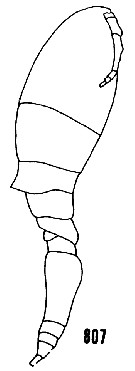 issued from : H.B. Owre & M. Foyo in Fauna Caribaea, 1, Crustacea, 1: Copepoda. Copepods of the Florida Current. 1967. [p.111, Fig.807]. As Oncaea conifera. After Giesbrecht (1892). Female: 807, habitus (lateral). Owre & Foyo (1964) reported that it was common at one Caribean station (SL 53) where the range was 100-1316 m but 84 p. cent of the catch came from 100-292 m.
|
 Issued from : G.A. Heron & J.M. Bradford-Grieve in New Zealand Oceanogr. Inst Memoir 104. NIWA, 1995. [p.18, Fig.4]. As Oncaea conifera. Female (from Gulf of Naples): a-b, habitus (lateral and dorsal, respectively) [q]; c, urosome (dorsal) [r]; d, segment of P5 and genital segment (lateral) [r]; e, left A1 [s]; f, left A2 [s]; g, labrum (ventral, exterior) [t]; h, labrum (interior) [t]; i, right Md [u]; j, left Mx1 [u]; k, right Mx2 [t]; l, right Mxp [u]. Scale bars in p.13, fig.2. Letter in brackets. Nota: P6 probably represented by spiniform setule on external genital area (fig.d)
|
 Issued from : G.A. Heron & J.M. Bradford-Grieve in New Zealand Oceanogr. Inst Memoir 104. NIWA, 1995. [p.19, Fig.5, a-d]. As Oncaea conifera. Female (from Gulf of Naples): a, P1 [v]; b, P2 [v]; c, P3 [v]; d, P4 [v] Scale bars in p.13, fig.2. Letter in brackets.
|
 Issued from : G.A. Heron & J.M. Bradford-Grieve in New Zealand Oceanogr. Inst Memoir 104. NIWA, 1995. [p.17]. As Oncaea conifera. Female: Armament of swimming legs P1 to P4. Si = inner border; Se = outer border; St = terminal border; Arabic numerals = setae; Roman numerals = spines. Nota: Legs 1-4 with serrate, hyaline flanges on spines. Endopods of legs 2-4 with conical process between 2nd and terminal spines.
|
 Issued from : G.A. Heron & J.M. Bradford-Grieve in New Zealand Oceanogr. Inst Memoir 104. NIWA, 1995. [p.19, Fig.5, e]. As Oncaea conifera. Female: e, P5 [s] Scale bar in p.13, Fig.2. Letter in brackets. Nota: P5 with oblong free segment, about 3 times as long as wide; 2 terminal setae, inner twice the length of outer; ratio of length of outer seta to that of segment 1.3:1; seta on body near leg
|
 Issued from : G.A. Heron & J.M. Bradford-Grieve in New Zealand Oceanogr. Inst Memoir 104. NIWA, 1995. [p.19, Fig.5, f-h]. As Oncaea conifera. Male (from Gulf of Naples): f, habitus (lateral) [r]; g, same (dorsal) [r]; h, left Mxp [s]. Scale bar in p.13, Fig.2. Letter in brackets.
| | | | | Ref. compl.: | | | Guangshan & Honglin, 1984 (p.118, tab.); Lapernat & Razouls, 2001 (tab.1); Böttger-Schnack & al., 2001 (p.1029, tab.1, 2); Krsinic & Grbec, 2002 (p.127, tab.1); Hsieh & al., 2004 (p.398, tab.1); Nishibe & Ikeda, 2004 (p.931, Tab. 2, 4, 5); Isari & al., 2006 (p.241, tab.II); Fernandes, 2008 (p.465, Tabl.2); McKinnon & al., 2008 (p.844: Tab.I, p.848: Tab. IV); Miyashita & al., 2009 (p.815, Tabl.II); Nishibe & al., 2009 (p.491, Table 1: seasonal abundance); Böttger-Schnack & Schnack, 2009 (p.131, Table 3, 4); C.E. Morales & al., 2010 (p.158, Table 1); Hernandez-Trujillo & al., 2010 (p.913, Table 2); Hidalgo & al., 2010 (p.2089, fig.2, 4, Table 2, cluster analysis); Dias & al., 2010 (p.230, Table 1, fig.6 b); Mazzocchi & Di Capua, 2010 (p.429); Dvoretsky & Dvoretsky, 2010 (p.991, Table 2); Andersen N.G. & al., 2011 (p.71, Fig.3: abundance); Isari & al., 2011 (p.51, Table 2, abundance vs distribution); Shiganova & al., 2012 §p.61, Table 4); Uysal & Shmeleva, 2012 (p.909, Table I); Salah S. & al., 2012 (p.155, Tableau 1); Lavaniegos & al., 2012 (p. 11, Table 1, fig.3, seasonal abundance, Appendix); Hidalgo & al., 2012 (p.134, Table 2, 3, figs.6, 8, occurrence vs hydrology) ; Gubanova & al., 2013 (in press, p.4, Table 2); Belmonte & al., 2013 (p.222, Table 2, abundance vs stations); Palomares-Garcia & al., 2013 (p.1009, Table I, abundance vs environmental factors); in CalCOFI regional list (MDO, Nov. 2013; M. Ohman, comm. pers.); Tachibana & al., 2013 (p.545, Table 1, seasonal change 2006-2008); Sano & al., 2013 (p.11, Table 2, feeding habits); Bonecker & a., 2014 (p.445, Table II: frequency, horizontal & vertical distributions); Lopez-Ibarra & al., 2014 (p.453, fig.6, biogeographical affinity); Fierro Gonzalvez, 2014 (p.1, Tab. 3, 4, 5, occurrence, abundance); Dias & al., 2015 (p.483, Table 2: abundance, biomasse, production; Table b4: % vs. seasonZakaria & al., 2016 (p.1, Table 1); Benedetti & al., 2016 (p.159, Table I, fig.1, functional characters); Ben Ltaief & al., 2017 (p.1, Table III, Summer relative abundance); Jerez-Guerrero & al., 2017 (p.1046, Table 1: temporal occurrence); El Arraj & al., 2017 (p.272, table 2, seasonal composition); Benedetti & al., 2018 (p.1, Fig.2: ecological functional group); Chaouadi & Hafferssas, 2018 (p.913, Table II: occurrence); Acha & al., 2020 (p.1, Table 3: occurrence % vs ecoregions). | | | | NZ: | 25 | | |
|
Carte de distribution de Triconia conifera par zones géographiques
|
| | | | | | | | | | | | | | | | | | 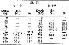 issued from : H.B. Owre & M. Foyo in Fauna Caribaea, 1, Crustacea, 1: Copepoda. Copepods of the Florida Current. 1967. [p.112, Table 54]. issued from : H.B. Owre & M. Foyo in Fauna Caribaea, 1, Crustacea, 1: Copepoda. Copepods of the Florida Current. 1967. [p.112, Table 54].
Vertical distribution of Oncaea (= Triconia) conifera at the ''40-Mile Station" in the Floruda Current (±25°35'N, 79°27'W).
SL 53: 18 V 1958; A: during midday, B: during midnight. |
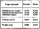 issued from : A.A. Shmeleva in Bull. Inst. Oceanogr., Monaco, 1965, 65 (n°1351). [Table 6: 42]. Oncaea conifera (from South Adriatic). issued from : A.A. Shmeleva in Bull. Inst. Oceanogr., Monaco, 1965, 65 (n°1351). [Table 6: 42]. Oncaea conifera (from South Adriatic).
Dimensions, volume and Weight wet. Means for 50-60 specimens. Volume and weight calculated by geometrical method. Assumed that the specific gravity of the Copepod body is equal to 1, then the volume will correspond to the weight. |
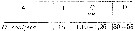 issued from : A.V. Kovalev in Gidrobiol. Zh., 1970,
6 (5). [p.92, Table 1]. As Oncaea conifera. issued from : A.V. Kovalev in Gidrobiol. Zh., 1970,
6 (5). [p.92, Table 1]. As Oncaea conifera.
Relation between the body length of females and number of eggs.
A: species; B: number of females; C: length of females in mm; D: number of eggs in relation to the lengths of females. |
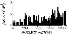 issued from : L.R. Haury & P.H. Wiebe in Deep-Sea Res., 1982, 29 (7A). [p.918, Fig.1, B]. issued from : L.R. Haury & P.H. Wiebe in Deep-Sea Res., 1982, 29 (7A). [p.918, Fig.1, B].
Abundance horizontal distribution of Oncaea (= Triconia) conifera: non-random spatial structure.
Samples collected with a Longhurst-Hardy Plankton Recorder (LHPR) in the northern Sargasso Sea (34°10'N; 71°35'W) at three depth stata.
Nota: The pattern reveal that dominant variations occurred on scales of tens to hundreds of meters. The fluctuations in abundance are evident on different scales simultaneously.
After the authors, the abundance of species was not significantly nor consistently correlated to either temperature or alinity on the scales resolved by the tows, thus the LHPR data indicate that the physical environment or depth changes along the horizontal tows, was not, in general, a direct causative factor for the patterns observed. |
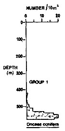 Issued from : R.K. Pipe & S.H. Coombs in J. Plankton Res., 1980, 2 (3). [p.230, Fig.4]. Issued from : R.K. Pipe & S.H. Coombs in J. Plankton Res., 1980, 2 (3). [p.230, Fig.4].
Oncaea conifera (= Triconia conifera) from Wyville Thomson Ridge (60°03.4' N, 07°03.9' W to 60°08' N, 07°02.9' W) on 24 April 1978: Vertical distribution.
Members of this group (Group 1) were restricted, for the most part, to Norwegian Sea Deep water at depths below 530 m in temperatures of 0-4.8°C.
This group contained 7 calanoids and 1 cyclopoid, plus 2 chaetognaths and 1 euphausid. The 2 most abundant species were S. abyssalis and Oncaea (= Triconia) conifera which together contributed over 75% of the specimen taken in the group. Their distributions showing peak abundance between 530 m and the bottom of the haul (580 m).
Euphausia norvegica euphhausid was attached to this group at a lower level of similarity (19%).
A computed coefficient of dissimilarity was used in association with a 'group-average' clustering strategy (see Clifford & Stephenson, 1975) to classify the plankton taxa on the basis of their vertical distribution after the indices of similarity and the results arranged diagramatically in the form of a dendogram (Fig.2). Classification was carried out using the Bray-Curtis measure which gives a coefficient of dissimilarity. |
| | | | Loc: | | | Cosmopolite. Also: Antarct. (Peninsula, Drake Passage, Atlant. (SW & S), Indian, Australia (North West Cape), Pacif. (SW, SE), Ross Sea), sub-Arct. (SW & SE Pacif.), Wyville Thomson Ridge, Barents Sea, Bering Sea (slope and shelf), St. Lawrence Island, N Baffin Sea, Anadyr Strait, G. of Thailand, Tioman Is. (Malaysia), Ambon Bay, W Channel of Korea Strait, Cheju Island, China Seas (Yellow Sea, East China Sea, South China Sea), Hong Kong, Taiwan Strait, Taiwan (E: Kuroshio Current, NE), Nagasaki, Korea Strait, Japan (Kuchinoerabu Is., Sagami Bay, Tosa Bay, Tokyo Bay, Kuroshio & Oyashio regions), Oregon (off Newport), Baja California (Bahia Magdalena, La Paz), Gulf of California, Bahia Cupica (Colombia), Galapagos-Ecuador, Peruvian shelf, off Chimbote, Chile (N-S, off Santiago). | | | | N: | 331 ? | | | | Lg.: | | | (11) F: 1,18; (25) F: 1,4-1,2; M: 0,75-0,65; (31) F: 1,2-1,15; (34) F: 1,2-1,15; (35) F: 1,38-1,16; ? (36) F: 1,12-1,33; M, 0,88-1; (38) F: 1,38-1,2; (45) F: 1,25-0,75; M: 0,8-0,6; (46) F: 1,23-1,15; M: 0,8-0,75; (36) F: 1,33-1,12; M: 1-0,88; (59) F: 1,4-0,75; M: 0,8-0,6; (104) F: 1,1; (109) F: 0,8-0,72; M: 0,76-0,72; (139) F: 1,29-0,98; M: 0,88-0,76; (142) F: 1,2; M ± 0,8; (180) F: 1,28-1,2; M: 0,86-0,8; (190) F: 0,65; (208) F: 1,5-0,8; M: 0,8; (237) F: 1,05-1,3; M: 0,7-1,0: (254) F: 1,06; M: 0,8; (327) F: 1,34-1,07; M: 0,79; (334) F: 1,25-0,75; M: 0,8-0,6; (340) M: 0,7; (432) F: 1,37-1,1; (449) F: 1,25-0,75; M: 0,8-0,6; (530) F: 1,2; M: 1,1; (531) F: 1,1; M: 0,8; (651) F: 1,16; (687) F: 1,26-1,01; M: 0,82-0,6; (788) F: 1,06-0,98; M: 0,7-0,62; (810) F: 1,06-0,98; M: 0,70-0,62; (864) F: 1-1,1; (920) F: 1,18; (991) F: 0,75-1,25; M: 0,60-0,80; (1023) F: 1-1,08; (1064) F: 1,12-1,28; M: 0,72-0,793; (1101) F: 1,11-1,25; {F: 0,65-1,50; M: 0,60-1,10}
The mean female size is 1.123 mm (n = 63; SD = 0.1929), and the mean male size is 0.7696 mm (n = 41; SD = 0.1208). The size ratio (male : female) is 0.685 or ± 69 %. | | | | Rem.: | épi à bathypélagique.
Sampling depth (Antarct., sub-Antarct.) : 0-1000 m. 0-3010 m at Station T-1 (E Tori Is., E middle Japan) from Furuhashi (1966 a). 420-580 m (Pipe & Coombs, 1980, Arctic: 60°N).
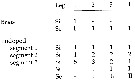
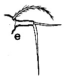
Giesbrecht (1902, p.41) considère l'existence de 3 variétés comme de simples différences ecophenotypiques du fait que Sars (1900, p.113) n'a pas donné une description d'exemplaires arctiques suffisamment pour permettre de créer une espèce nouvelle. Les différences entre les variétés dans les différentes mers: variété 1 (Méditerranée, Pacifique), variété 2 (Arctique) et variété 3 (Antarctique). Chacune des 3 variétés montre des caractéristiques propres. La variété I a une longueur corporelle (a) comprise entre 1, 15 et 1,23; la longueur du segment génital (b) est 1,5 la longueur du reste de l'abdomen; le segment génital (c) est renflé ventralement; la furca (d) n'et pas plus longue que le segment anal et 2 à 2,5 fois aussi longue que large (e); la P5 (f) est 3 fois plus longue que large.
La variété II a une longueur corporelle comprise entre 0.7 et 0,75; le segment génital est aussi long que le reste de l'abdomen et plutot plat; la furca est 2 fois aussi longue que large; la P5 est plus longue que large. La variété III a une longueur corporelle de 1,1 à 1,25; le segment génital est aussi long que le reste de l'abdomen et presque plat;, la furca est 4 fois aussi longue que large; la P5 est à peine plus longue que large. la longueur de la furca est 1 fois i/3 celle du segment anal.
Les caractères s'accordent pour c et d dans les variétés 1 et 2.
Les différences portent sur les longueurs corporelle dans les variétés 1 et 3.
Les différences portent sur les caractères b, c et f dans les variétés 2 et 3.
les espèces polaires se distinguent de la variété 1 par une partie seulement de leur variation b, c, f; une aurtre remarque est que la variété arctique est plus petite et la variété antarctique plus grande.
Ultérieurement il a été étabi que la variété III est une espèce nouvelle Oncaea (= Triconia) antarctica Giesbrecht, 1902.
Voir aussi les remarques en anglais | | | Dernière mise à jour : 25/10/2022 | |
|
|
 Toute utilisation de ce site pour une publication sera mentionnée avec la référence suivante : Toute utilisation de ce site pour une publication sera mentionnée avec la référence suivante :
Razouls C., Desreumaux N., Kouwenberg J. et de Bovée F., 2005-2026. - Biodiversité des Copépodes planctoniques marins (morphologie, répartition géographique et données biologiques). Sorbonne Université, CNRS. Disponible sur http://copepodes.obs-banyuls.fr [Accédé le 30 mars 2026] © copyright 2005-2026 Sorbonne Université, CNRS
|
|
|
|


;)
;)
;)
;)
;)
;)
;)
;)
;)
;)
;)
;)
;)
;)
;)
;)
;)
;)
;)
;)
;)
;)
;)
;)
;)
;)
;)
;)
;)
;)
;)
;)

;)
;)
;)
;)