|
|
 |
Fiche d'espèce de Copépode |
|
|
Calanoida ( Ordre ) |
|
|
|
Clausocalanoidea ( Superfamille ) |
|
|
|
Clausocalanidae ( Famille ) |
|
|
|
Clausocalanus ( Genre ) |
|
|
| |
Clausocalanus farrani Sewell, 1929 (F,M) | |
| | | | | | | Syn.: | Clausocalanus arcuicornis minor Brodsky, 1962 c (part., p.116, figs.F); Grice, 1962 (p.189, pl.7, figs.5,6: F);
Clausocalanus pergens : Mori, 1937 (1964) (pl.14, figs.2-5); Fleminger, 1964 a; 1967 a (tab. I); Chen & Zhang, 1965 (p.49, figs.F); Kos, 1972 (Vol.1, figs. partim) | | | | Ref.: | | | Sewell, 1929 (p.94, Descr.F, figs.F); Farran, 1936 a (p.81, Rem.); Sewell, 1947 (p.55); Frost & Fleminger, 1968 (p.52, Descr.M, figs.F,M, Rem.); Silas, 1972 (p.646); ? Chen & Zhang, 1974 (p.103, 111, figs.M); Dawson & Knatz, 1980 (p.7, figs.F,M); Chahsavar-Archad & Razouls, 1982 (p.37, fig.F); van der Spoel & Heyman, 1983 (p.44, fig.56); Chihara & Murano, 1997 (p.776, Pl.89,94: F,M); Bucklin & al., 2003 (p.335, tab.2, fig.1, Biomol) | 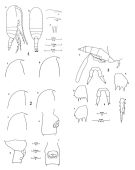 issued from : B. Frost & A. Fleminger in Bull. Scripps Inst. Oceanogr. Univ. California, San Diego, 1968, 12. [Pl.34, p.168-169; Pl.35, p.170-171; Pl.6, p.172-173]. Female: 1 a, habitus (right lateral view); 1 b, idem (dorsal view); 1 c-d, rostrum (right lateral); 1 e, rostrum (anteroventral); 1 f-g, frontal region (right lateral; 1 a-c taken from different specimens; 1 d-e from a fourth; 1 f and g from fifth and sixth specimens respectively; 2 a-c, frontal region (right lateral); 2 d, Th.3 (posterior part), Th.4-5 and genital segment (right lateral); 2 e, genital segment (right lateral); 2 f, genital segment (ventral view); 2 a-f taken from different specimens; 3 a, Th.4-5 (posterior part) and urosome with spermatophore attached; 3 b, B2 of P2; 3 c-d, B2 of P3; 3 e, Re3 and St of P3; 3 f-g, P5; 3 a from one specimen; 3 b,c,e from another; 3 d, f, g from third, fourth and fifth specimens, respectively.
|
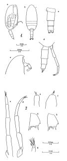 issued from : B. Frost & A. Fleminger in Bull. Scripps Inst. Oceanogr. Univ. California, San Diego, 1968, 12. [Pl.37, p.174-175; Pl.38, p.176-177]. Male: 1 a, habitus (right lateral view); 1 b, idem (dorsal view); 1 c, frontal region (right lateral); 1 d, Th.4-5 (posterior part) and urosome (right lateral); 1 e, urosome (dorsal view); 1 a-e taken from different specimens; 2 a, B2 of P2; 2 b, B2 of P3; 2 c, P5 (posterior); 2 d, P5 (right lateral); 2 e, right P5 (anterior); 2 f, right P5 (right lateral); 2 g, 4P5 (distal part) and 5P5 (posterior); 2 a-b taken from one spegimen; 2 c,e from another; 2 d,f,g from a third.
|
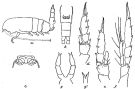 issued from : R.B.S. Sewell in Mem. Indian Mus., 1929, X. [p.94, Fig.38]. Female (from S India): a, habitus (lateral left side); b, urosome (ventral); c, genital opening; d, P2; e, P3; f, P4; g, P5; g', the end of distal segment of P5 (enlarged).
|
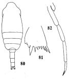 issued from : Q.-c Chen & S.-c. Zhang in Studia Marina Sinica, 1974, 9. [Pl.7, Figs.80-823]. Doubtful. Male (from South China Sea): 80, habitus (dorsal); 81, basipodite 2 of P2; 82, P5.
|
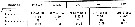 issued from : B. Frost & A. Fleminger in Bull. Scripps Inst. Oceanogr. Univ. California, 1968, 12. [p.46, Table 3a]. Clausocalanus farrani Females: Measurements and ratios . TL = total body length ; SL = spermatophore length ; P :U = ratio of prosome length to urosome length ; U :U1 = ratio of total urosome length to length of 1st urosomal segment (genital segment) ; S :U1 = ratio of spermatophore sac length to U1 length of female on which spermatophore is attached ; r = sample range; m = sample mean; n = number of specimens measured; s = sample standard deviation.
|
 issued from : B. Frost & A. Fleminger in Bull. Scripps Inst. Oceanogr. Univ. California, 1968, 12. [p.47, Table 3b]. Clausocalanus farrani Males: Measurements and ratios . TL = total body length; P :U = ratio of prosome length to urosome length ; P:U2 = ratio of prosome length to length od 2nd urosomal segment; U2:2P5 = ratio of U2 length to length of 2nd segment of longer ramus of P5; U2:3P5 = ratio of U2 length of 3rd segment of longer ramus of P5; 3P5:2P5 = ratio of length of 3P5 of longer ramus to length of 2P5 of longer ramus; r = sample range; m = sample mean; n = number of specimens measured; s = sample standard deviation.
|
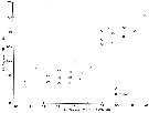 issued from : B. Frost & A. Fleminger in Bull. Scripps Inst. Oceanogr. Univ. California, 1968, 12. [p.25, Fig.8]. Ratio of length of A1 fused segments 20-21 to length of A1 segment 22 (ordinate) plotted against length of A1 fused segments 20-21 (abscissa) for males of Clausocalanus farrani and C. minor.
|
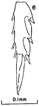 issued from : B. Frost & A. Fleminger in Bull. Scripps Inst. Oceanogr. Univ. California, 1968, 12. [p.173, Pl.36, e]. Female: e, exopodal segment 3 and terminal seta of P3.
|
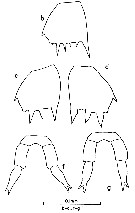 issued from : B. Frost & A. Fleminger in Bull. Scripps Inst. Oceanogr. Univ. California, 1968, 12. [p.173, Pl.36, b, c-d, f-g]. Female: b, basipodite 2 of P2; c-d, basipodite 2 of P3, f-g, P5 (from different specimens).
|
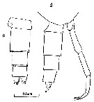 issued from : B. Frost & A. Fleminger in Bull. Scripps Inst. Oceanogr. Univ. California, 1968, 12. [p.175, Pl.37, d, e]. Male: d, posterior part of last thoracic segment and urosome (right lateral); e, urosome (dorsal).
|
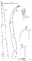 issued from : B. Frost & A. Fleminger in Bull. Scripps Inst. Oceanogr. Univ. California, 1968, 12. [p.177, Pl.38, c-d, e-f, g]. Male: c, P5 (posterior); d, P5 (right lateral); e, right P5 (anterior); f, right P5 (right lateral); g, 4th segment of P5 (distal part) and 5th segment of P5 (posterior).
|
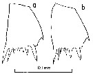 issued from : B. Frost & A. Fleminger in Bull. Scripps Inst. Oceanogr. Univ. California, 1968, 12. [p.177, Pl.38, a, b]. Male: a, basipodite 2 of P2; b, basipodite 2 of P3.
|
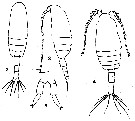 Issued from : T. Mori inThe pelagic Ciopepoda from the neighbouring waters of Japan, 1964 (1937). [Pl. 14, Figs. 2-5] As Clausocalanus pergens. After Frost & Fleminger, 1968 (p.52) : Syn. from Clausocalanus farrani. Female (from Japan ): 2, habitus (dorsal); 3, same (lateral); 5, P5. Male: 4, habitus (dorsal).
| | | | | Ref. compl.: | | | Grice & Hulsemann, 1967 (p.14); Fleminger, 1967 a (tabl.1); Björnberg, 1973 (p.310, 385); Fleminger & Hulsemann, 1973 (p.340, carte); Timonin, 1976 (p.79, vertical distribution); Timonin & Voronina, 1977 (p.288, fig.6); Carter, 1977 (1978) (p.35); Star & Mullin, 1981 (p.1322, abundance); Smith S.L., 1982 (p.1331, abundance, monsoon effect); Almeida Prado Por, 1983 (p.141, tab.); Guangshan & Honglin, 1984 (p.118, tab.); Binet, 1984 (tab.3); 1985 (p.85, tab.3); Almeida Prado Por, 1985 (p.250); Brinton & al., 1986 (p.228, Table 1); Madhupratap & Haridas, 1986 (p.105, tab.1); Jimenez-Perez & Lara-Lara, 1988; Echelman & Fishelson, 1990 a (tab.2); Hirakawa & al., 1990 (tab.3); Yoo, 1991 (tab.1); Shih & Young, 1995 (p.72); Noda & al., 1998 (p.55, Table 3, occurrence); Suarez-Morales & Gasca, 1998 a (p109); Lavaniegos & Gonzalez-Navarro, 1999 (p.239, Appx.1); Hsiao & al., 2004 (p.325, tab.1); Lan & al., 2004 (p.332, tab.1); Lo & al., 2004 (p.89, tab.1); Kazmi, 2004 (p.229); Smith & Madhupratap, 2005 (p.214, tab.4); Cornils & al., 2007 (p.1261, feeding); Cornils & al., 2007 (p.57, Table I, fig.2, Rem: reproduction; abnormality); Valdés & al., 2007 (p.103: tab.1); Dur & al., 2007 (p.197, Table IV); McKinnon & al., 2008 (p.844: Tab.1, p.846: Tab.II,); Cabal & al., 2008 (289, Table 1); Lan Y.C. & al., 2008 (p.61, Table 1, % vs stations); C.-Y. Lee & al., 2009 (p.151, Tab.2); Lan Y.-C. & al., 2009 (p.1, Table 2, % vs hydrogaphic conditions); Cornils & al., 2010 (p.2076, Table 3); Hsiao S.H. & al., 2011 (p.475, Appendix I); Hsiao & al., 2011 (p.317, Table 2, indicator of seasonal change); Pillai H.U.K. & al., 2011 (p.239, Table 3, vertical distribution); Tutasi & al., 2011 (p.791, Table 1, 3, fig.9, abundance distribution vs La Niña event, Rem. p.797, fig.11);in CalCOFI regional list (MDO, Nov. 2013; M. Ohman, comm. pers.); Tachibana & al., 2013 (p.545, Table 1, seasonal change 2006-2008); Tseng & al., 2013 (p.507, seasonal abundance); Hirai & al., 2013 (p.1, Table I, molecular marker); Lidvanov & al., 2013 (p.290, Table 2, % composition); Zaafa & al., 2014 (p.67, Table I, occurrence); El Arraj & al., 2017 (p.272, table 2, spatial distribution); Palomares-Garcia & al., 2018 (p.178, Table 1: occurrence); | | | | NZ: | 13 | | |
|
Carte de distribution de Clausocalanus farrani par zones géographiques
|
| | | | | | | | | | | | 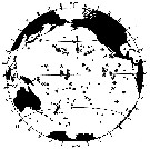 issued from : B. Frost & A. Fleminger in Bull. Scripps Inst. Oceanogr. Univ. California, San Diego, 1968, 12. [p.54, Chart 6, a]. issued from : B. Frost & A. Fleminger in Bull. Scripps Inst. Oceanogr. Univ. California, San Diego, 1968, 12. [p.54, Chart 6, a].
Occurrence of C. farrani in samples examined; closed circles represent samples examined; open circles represent samples in which adults were found; bars through open circles represent samples from which specimens were removed for measurements. |
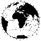 issued from : B. Frost & A. Fleminger in Bull. Scripps Inst. Oceanogr. Univ. California, San Diego, 1968, 12. [p.55, Chart 6, b]. issued from : B. Frost & A. Fleminger in Bull. Scripps Inst. Oceanogr. Univ. California, San Diego, 1968, 12. [p.55, Chart 6, b].
Occurrence of C. mastigophorus in samples examined; closed circles represent samples examined; open circles represent samples in which adults were found; bars through open circles represent samples from which specimens were removed for measurements. |
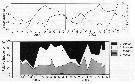 issued from : A. Cornils, B. Niehoff, C. Richter, T. Al-Najjar & B. Schnack-Schiel in J. Plankton Res., 2007, 29 (1). [p.60, Figs.1, 2]. issued from : A. Cornils, B. Niehoff, C. Richter, T. Al-Najjar & B. Schnack-Schiel in J. Plankton Res., 2007, 29 (1). [p.60, Figs.1, 2].
Above: Annual cycle of sea surface temperature and depth -integrated (0-100 m) chlorophyll a (mg/m2)
Below: Relative frequency (%) of the clausocalanid females over the investigation period (March 2002 to December 2003) in the northern Gulf of Aqaba (29°27'87 N, 34°57' 87 E; depth 300 m) for Clausocalanus farrani, C. furcatus, C. minor and Ctenocalanus vanus.
Nota: Collected by vertical hauls from 100 m depth to the surface. Sampling performed between 9 a.m. and 3 p.m. on a monthly basis. |
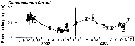 issued from : A. Cornils, B. Niehoff, C. Richter, T. Al-Najjar & B. Schnack-Schiel in J. Plankton Res., 2007, 29 (1). [p.65, Fig.8]. issued from : A. Cornils, B. Niehoff, C. Richter, T. Al-Najjar & B. Schnack-Schiel in J. Plankton Res., 2007, 29 (1). [p.65, Fig.8].
Prosome length (mm) displayed with SE bars over the investigation period. |
 issued from : A. Cornils, B. Niehoff, C. Richter, T. Al-Najjar & B. Schnack-Schiel in J. Plankton Res., 2007, 29 (1). [p.65, Table III]. issued from : A. Cornils, B. Niehoff, C. Richter, T. Al-Najjar & B. Schnack-Schiel in J. Plankton Res., 2007, 29 (1). [p.65, Table III].
Percentage of clausocalanid females infected with Blastodinium sp. (dinoflagellate) or showing abnormalities of the P5 (%), found in the preserved females. |
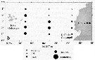 Issued from : P. Tutasi, S. Palma & M. Caceres in Scienc. Mar., 2011, 75 (4). [p.799, Fig.9 b] Issued from : P. Tutasi, S. Palma & M. Caceres in Scienc. Mar., 2011, 75 (4). [p.799, Fig.9 b]
Geographic distribution of Clausocalanus farrani in September and October 2001, associated with the weak La Niña event of 2001. |
| | | | Loc: | | | South Africa (E) (Natal), off Cape Verde Is. (in Chasavar-Archad & Razouls, 1982), Morocco-Mauritania, off W Tangier (in Zaafa & al., 2014), off Amazon, E Medit. (Lebanon coast)*, Red Sea (G. of Aqaba), Somalia, Arabian Sea, Indian, Andaman Sea (Barren Island) Australia (North West Cape), S Burma, SW Celebes, China Seas (Yellow Sea, East China Sea, South China Sea), Taiwan Strait, Taiwan (SW, E, NW, NE, N, Mienhua Canyon), Japan, Kuchinoerabu Is., Tokyo Bay, off S Baja California, G. of California, La Paz, W Mexico, Hawaii, Pacif. (E & W equatorial), Pacif. (N Central Gyre), Australia (Great Barrier), New Caledonia, Pacif. (sub-tropical), Chile.
* according to Almeida Prado Por, 1983 (C.R.: original document not seen). | | | | N: | 67 | | | | Lg.: | | | (29) F: 1,08-0,87; (30) F:1,2-1,04; M: 0,99-0,87; (34) F: 1,22-1,09; (109) M: 0,85-0,65; (290) F: 1,2-1; (338) M: 0,7-0,65; {F: 0,87-1,22; M: 0,65-0,99}
The mean female size is 1.088 mm (n = 8; SD = 0.1196) and the mean male size is 0.785 mm (n = 6; SD = 0.1394). The size ratio (male : female) is establish on one sample with males and females: 0.83. | | | | Rem.: | Les localisations atlantiques nécessitent une confirmation bien que Calef & Grice (1967) l'aient signalé au large de la Guyane.
* d'après Almeida Prado Por, 1983 (C.R.: document original non vu).
Voir aussi les remarques en anglais | | | Dernière mise à jour : 25/10/2022 | |
|
|
 Toute utilisation de ce site pour une publication sera mentionnée avec la référence suivante : Toute utilisation de ce site pour une publication sera mentionnée avec la référence suivante :
Razouls C., Desreumaux N., Kouwenberg J. et de Bovée F., 2005-2026. - Biodiversité des Copépodes planctoniques marins (morphologie, répartition géographique et données biologiques). Sorbonne Université, CNRS. Disponible sur http://copepodes.obs-banyuls.fr [Accédé le 22 mars 2026] © copyright 2005-2026 Sorbonne Université, CNRS
|
|
|
|




;)
;)
;)
;)
;)
;)
;)
;)
;)
;)
;)
;)
;)

;)
;)
;)
;)
;)
;)