|
|
 |
Fiche d'espèce de Copépode |
|
|
Calanoida ( Ordre ) |
|
|
|
Clausocalanoidea ( Superfamille ) |
|
|
|
Clausocalanidae ( Famille ) |
|
|
|
Ctenocalanus ( Genre ) |
|
|
| |
Ctenocalanus vanus Giesbrecht, 1888 (F,M) | |
| | | | | | | Syn.: | ? Ctenocalanus longicornis Mori, 1937 (1964) (p.37, figs.F); Delalo, 1968 (p.137, Rem.: ?); Andronov & Maigret, 1980 (p.71, Table 2, 3); Suarez-Morales & Gasca, 1998 a (p109); Hernandez-Trujillo & Esqueda-Escargera, 2002 (in Appendix); Ohtsuka & al., 2015 (p.123, Table 2);
no Ctenocalanus vanus (F) : ? Giesbrecht, 1902 (p.19); Ramirez, 1966 (p.12, figs.F); ? Arcos, 1976 (p.85, Rem.: p.91, Table II); ? Fukuchi & Tanimura, 1981 (p.37); ? Hoshiai & Tanimura, 1981 (p.44); ? Kawaguchi & al., 1986 (tab.2);
Ctenocalanus : Harris & al., 1986 (p.845, Table 2, comparison pump vs. net);
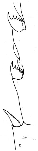
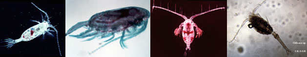
Ctenocalanus vanus s.l. : Brinton & al., 1986 (p.228, Table 1) | | | | Ref.: | | | Giesbrecht, 1892 (p.194, 772, figs.F); Giesbrecht & Schmeil, 1898 (p.28, Rem. F); Farran, 1908 b (p.28); ? Wolfenden, 1911 (p.203); Pesta, 1920 (p.506); Esterly, 1924 (p.91, figs.F,M); Farran, 1926 (p.241); 1929 (part., p.208, 226); Dakin & Colefax, 1933 (p.205); Rose, 1933 a (p.83, figs.F,M); Farran, 1936 a (p.85); Tanaka, 1937 (p.253, figs.F, Rem.); Dakin & Colefax, 1940 (p.97, figs.F,M); Brodsky, 1950 (1967) (p.121, figs.F,M); ? Vervoort, 1951 (? part., p.59); ? 1957 (p.37, Rem.); Tanaka, 1956 c (p.384, Rem.); Marques, 1958 (p.209); ? Tanaka, 1960 (p.35); Vervoort, 1963 b (p.119, Rem.); Björnberg, 1963 (p.34); Tanaka, 1964 (p.7); Vilela, 1965 (p.7); Park, 1968 (p.542); Vilela, 1968 (p.16, figs.F); Corral Estrada, 1970 (p.149); Bradford, 1972 (p.36, figs.F); Björnberg, 1972 (p.23, figs., Rem.N); Razouls, 1972 (p.94, Annexe: p.37, figs.F,M); Chen & Zhang, 1974 (p.112, figs.F,M); Séret, 1979 (p.55, figs.F); Dawson & Knatz, 1980 (p.6, figs.F,M); Björnberg & al., 1981 (p.629, figs.F,M, Rem.); Gardner & Szabo, 1982 (p.188, figs.F,M); Brodsky & al.,1983 (p.237, figs.F,M); Prado-Por, 1984 (p.87, 88, Rem.); Roe, 1984 (p.356); Sazhina, 1985 (p.46, figs.N); Vega-Pérez & Bowman, 1992, p.100, Rem.); Razouls, 1994 (p.50, figs.F,M); Bradford-Grieve, 1994 (p.125, figs.F,M, p.152, fig.101); Chihara & Murano, 1997 (p.778, Pl.88: F,M); Bradford-Grieve al., 1999 (p.878, 917, figs.F,M); Suarez-Morales & Leon-Oropeza, 2000 (p.39, tab.1, Rem.); Bucklin & al., 2003 (p.335, tab.2, fig. 4 Biomol); Avancini & al., 2006 (p.83, Pl. 52, figs.F,M, Rem.); Vives & Shmeleva, 2007 (p.627, figs.F,M, Rem.) | 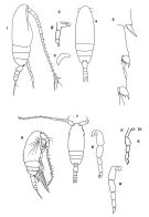 Female: 1, habitus (lateral); 2, P5 (regressed); issued from : Razouls C., 1972. 3, P5; issued from Giesbrecht, 1892. 4, habitus (dorsal); issued from Séret C. 5, exterior spine of Exopodide 2 and 3 of P4; issued from Heron & Bowman, 1971. Male: 6, habitus (lateral); issued from : Björnberg and al., 1981. 7, habitus (dorsal); 8, 8', P5 (from two samples for the Mediterranean Sea); issued from Razouls C., 1972. 9, P5 (G: left, Dt: right); issued from : Ramirez, 1966.
|
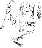
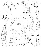
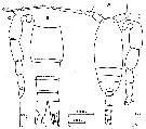
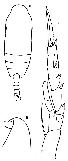
 issued from : F.C. Ramirez in Bol. Inst. Biol. Mar., Mar del Plata, 1966, 11. [Lam.V, Figs.1-15] Male (from off Mar del Plata): 1, P1; 2, habitus (dorsal); 3, posterior part cephalothorax and urosome; 4, urosome; 6, habitus (lateral right side); 7, P4 (spines of 3rd exopodal segment); 8, P2 (basipodal segment 2); 10, P3; 13, A1; 14, 1st segment of P5; 15, P5. Female: 3, P4 (spines of 3rd exopodal segment); 5, urosome (lateral left side); 9, habitus (dorsal); 11, P3 (basipodal segment 2); 12, P3 (spines of 3rd exopodal segment).
|
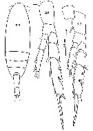
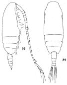 issued from : Q.-c Chen & S.-z. Zhang in Studia Marina Sinica, 1974, 9. [Pl.7, Figs.89-90]. Female (from South China Sea): 89, habitus (dorsal); 90, idem (lateral right side).
|
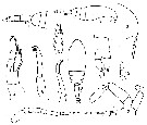
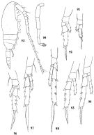 issued from : Q.-c. Chen & S.-z. Zhang in Studia Marina Sinica, 1974, 9. [Pl.8, Figs.91-99. Female: 91, P1; 92, P2; 93, P3; 94, P4. Male: 95, habitus (lateral right side); 96, P2; 97, P3; 98, P4; 99, P5.
|
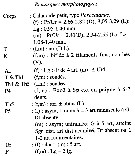
 issued from : T. Mori in The pelagic Copepoda from the neighbouring waters of Japan, 1937 (2nd edit., 1964). [Pl.15, Figs.8-16]. As Ctenocalanus longicornis. With doubt.. Female: 8, P2; 9, exopodite 3 of P3; 10, P3; 11, Md; 12, Md (masticatory edge); 13, P4; 14, urosome (dorsal); 15, A2; 16, habitus (lateral). Nota: Allied to C. vanus Giesbrecht, but P5 absent. A1 24-segmented; 8th and 9th segments fused; extending beyond the the body end by the terminal 3 segments. Only females obtained in the Ki-Channel (33°50'N, 134°E) in the summer. Body length about 1.23 mm.
|
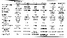 issued from : E. Suarez M. & A. Leon-Oropeza in Gulf and Caribbean Researc, 2000, 12. [p.39, Table I]. Characters used to separate the known species of Ctenocalanus. c/u ratio = cephalosome/urosome length ratio.
|
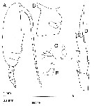
 issued from : C.O. Esterly in Univ. Calif. Publs Zool., 1924, 26 (5). [p.91, Fig.D). Female (from San Francisco Bay): 1, forehead (ventral); 2, habitus (lateral); 3, genital segment with seminal receptacle (ventral); 4, 3rd exopodal sement of P3; 5, anal segment and caudal rami ( specimen of La Jolla); 6, forehead (lateral); 7, caudal rami; 8, habitus (dorsal); 9, Mxp; 10, 3rd segment of exopod of P3 (a different specimen than in 4); 11, P3 (from a third specimen); 12, P5 (specimen from La Jolla); 13, A2; 14, A1; 15, first two segments of abdomen (lateral); 16, 3rd segment of exopod of P4.
|
 issued from : C.O. Esterly in Univ. Calif. Publs Zool., 1924, 26 (5). [p.92, Fig.E). Male: 1, last two thoracic segments and urosome (lateral, right side); 2, habitus (lateral); 3, forehead (lateral); 4, P1; 5, P5 (only left leg) ; 6, 3rd segment of exopod of P3; 7, P5 (another view); 8, habitus (dorsal); 9, last two abdominal segments and caudal rami (ventral); 10, P5 from immature specimen; 11, A1; 12, A2. Nota: According to Wolfenden (1904, p.104) right P5 represented by a very short stump.
|
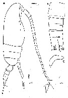
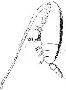 Issued from : W. Giesbrecht in Systematik und Faunistik der Pelagischen Copepoden des Golfes von Neapel und der angrenzenden Meeres-Abschnitte. Fauna Flora Golf. Neapel, 1892. Atlas von 54 Tafeln. [Taf.36, Fig.28]. Female: 28, habitus (lateral).
|
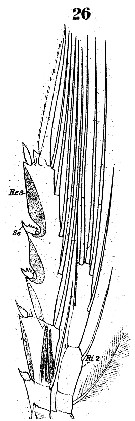 Issued from : W. Giesbrecht in Systematik und Faunistik der Pelagischen Copepoden des Golfes von Neapel und der angrenzenden Meeres-Abschnitte. Fauna Flora Golf. Neapel, 1892. Atlas von 54 Tafeln. [Taf.10, Fig.26]. Female: exo (Re) and endopod (Ri) of P1.
|
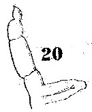 Issued from : W. Giesbrecht in Systematik und Faunistik der Pelagischen Copepoden des Golfes von Neapel und der angrenzenden Meeres-Abschnitte. Fauna Flora Golf. Neapel, 1892. Atlas von 54 Tafeln. [Taf.10, Fig.20]; Female: P5.
|
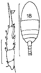 issued from : J.M. Bradford in Mem. N. Z. Oceonogr. Inst., 1972, 54. [p.35, Fig.5 (17-18)]. Female (from Kaikoura, New Zealand): 17, exopod of P3; 18, habitus (dorsal). Scale bars: 1 mm (18); 0.1 mm (17).
|
 issued from : C. Razouls in Th. Doc. Etat Fac. Sc. Paris VI, 1972, Annexe. [Fig.39]. Female (from Banyuls, Gulf of Lion): A, habitus (lateral, right side); B, urosome (dorsal); C, P5.
|
 issued from : C. Razouls in Th. Doc. Etat Fac. Sc. Paris VI, 1972, Annexe. [Fig.40]. Male: A, habitus (dorsal); B, urosomal segments 2-5 (dorsal); C, P5; D, P5 (another specimen).
|
 issued from : G.A. Heron & T.E. Bowman in Biology Antarctic Seas IV. Antarct. Res. Ser., 1971, 17. [p.142, Fig.2].Female (from 29°N, 80°32.7'W): outer spine of exopod 2 and proximal outer spines of exopod 3 of P4.
|
 issued from : J.M. Bradford-Grieve in The Marine Fauna of New Zealand: Pelagic Calanoid Copepoda. National Institute of Water and Atmospheric Research (NIWA). New Zealand Oceanographic Institute Memoir, 102, 1994. [p.126, Fig.73, F-I]. Female (from 36°18'S, 174°56'E): F, habitus (lateral); G, basipod 2 (= basis) of P2; H, basipod 2 (= basis) of P3; I, P5.
|
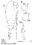 issued from : J.M. Bradford-Grieve in The Marine Fauna of New Zealand: Pelagic Calanoid Copepoda. National Institute of Water and Atmospheric Research (NIWA). New Zealand Oceanographic Institute Memoir, 102, 1994. [p.126, Fig.73, F-I]. Male (from 36°18'S, 174°56'E): F, habitus (lateral); G, basipod 2 (= basis) of P2; H, basipod 2 (= basis) of P3; I, P5.
|
 Issued from : O. Tanaka in Japanese J. Zool., 1937, VII, 13. [p.253, Fig.3]. Female (from coast of Heda, Japan): a, habitus (dorsal); b, forehead (lateral); c, P3. Nota: Cephalothorax 0,93 mm; abdomen: 0.34 mm.
|
 Issued from : C. Séret in Thesis UPMC, Paris 6. 1979 [Pl. VIII, figs.44-46]. Female (from off N Kerguelen Is.): 44, habitus (dorsal); 45, P3; 46, P. Nota: Cephalosome 2.5 times longer than abdomen. Caudal rami 2.7 times longer than wide.
|
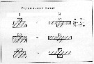
 Issued from : C. Séret in Thesis UPMC, Paris 6. 1979 [Tableau VII, p.58]. Number of indentation from first and second outer spines in swimming legs P3 and P4 in Ctenocalanus.
|
 Issued from : C. Razouls in Ann. Inst. océanogr., Paris, 1994, 70 (1). [p.50]. Caractéristiques morphologiques de Ctenocalanus vanus femelle et mâle adultes. Terminologie et abbréviations: voir à Calanus propinquus. Nota: Peut être confondu avec Ctenocalanus citer notamment dans la littérature avant 1971. L'exemplaire femelle de Méditerranée (Banyuls-sur-Mer) présente les proportions suivantes de l'urosome (%): 31, 9 : 19,1 : 14,9 : 16 : 18 . F: Lg/lg = 1.8. La P5 montre diverses variations, et parfois difficile à observer. Chez le mâle, la P5 relativement grande, montre également une certaine variabilité
| | | | | Ref. compl.: | | | Pearson, 1906 (p.10); Rose, 1925 (p.152); ? Hardy & Gunther, 1935 (1936) (p.149, Rem.); Sewell, 1948 (p.345, 395, 400, 407, 422, 431, 450, 453, 455, 469, 495, 497, 499, 513, 522, 555, 559); Grice & Hart, 1962, table 4: abundance); Gaudy, 1962 (p.93, 99, Rem.: p.105); ? Senô & al., 1963 a (p.4, 5); Duran, 1963 (p.15); V.N. Greze, 1963 a (tabl.2); Shmeleva, 1963 (p.141); Ahlstrom & Thrailkill, 1963 (p.57, Table 5, abundance); Grice, 1963 a (p.495); Gaudy, 1963 (p.22, Rem.); Björnberg, 1963 (p.34, Rem.); De Decker, 1964 (p.15, 20, 29); Unterüberbacher, 1964 (p.20, Rem.); De Decker & Mombeck, 1964 (p.12); Grice & Hulsemann, 1965 (p.223); Shmeleva, 1965 b (p.1350, lengths-volume -weight relation); Pavlova, 1966 (p.43); ? Senô & al., 1966 (p.4, 5); Furuhashi, 1966 a (p.295, vertical distribution vs mixing Oyashio/Kuroshio region, Table 10); Neto & Paiva, 1966 (p.23, Table III); Mazza, 1966 (p.70); 1967 (p.355: Rem.); Grice & Hulsemann, 1967 (p.14); De Decker, 1968 (p.45); Delalo, 1968 (p.137); Champalbert, 1969 a (p.635); Itoh, 1970 (tab.1); Park, 1970 (p.475); Deevey, 1971 (p.224); Gamulin, 1971 (p.381, tab.2, 3); Carli, 1971 (p.372, tab.1); Paulmier, 1971 (p.168); Lefèvre-Lehoërff, 1972 (p.1681); Binet & al., 1972 (p.69); Roe, 1972 (p.277, tab.1, 2); Apostolopoulou, 1972 (p.327, 345); Bainbridge, 1972 (p.61, Appendix Table I: vertical distribution vs day/night); Binet, 1973 (p.77); Björnberg, 1973 (p.317, 385); Corral Estrada & Pereiro Muñoz, 1974 (tab.I); Vives & al., 1975 (p.41, tab.II, III, IV); Peterson & Miller, 1975 (p.642, 650, Table 3, interannual abundance); 1976 (p.14, Table 1, 2, 3, abundance vs interannual variations); Deevey & Brooks, 1977 (p.256, tab.2, Station "S"); Grindley, 1977 (p.341, Table 2); Peterson & Miller, 1977 (p.717, Table 1, seasonal occurrence); Carter, 1977 (1978) (p.35); Nyan Taw & Ritz, 1979 (p.196); Porumb, 1980 (p.168); Vaissière & Séguin, 1980 (p.23, tab.1); Kovalev & Schmeleva, 1982 (p.83); Vives, 1982 (p.290); Brenning, 1982 a (p.14, spatial distribution & T-S diagram, Rem.); De Decker, 1984 (p.315, 345: chart); Scotto di Carlo & al., 1984 (p.1041); Binet, 1984 (tab.3); Brenning, 1985 a (p.24, Table 2); Kimmerer & McKinnon, 1985 (p.149); Regner, 1985 (p.11, Rem.: p.29); Jansa, 1985 (p.108, Tabl.I, , II, III, IV); Valentin & al., 1986 (p.117, temporal variations); Yamada & Kawamura, 1986 (p.86, Table 4); ? Zmijewska, 1987 (tab.2a); Lozano Soldevilla & al., 1988 (p.58); Hirakawa & al., 1990 (tab.3); Hattori, 1991 (tab.1, Appendix); Yoo, 1991 (tab.1); Hirakawa, 1991 (p.376: fig.2); Fernandez Araoz, 1991 (p.575); Santos & Ramirez, 1991 (p.79, 80, 82, 83); Hays & al., 1994 (tab.1); Kouwenberg, 1994 (tab.1); Verheye & al., 1994 (p.155); Hirakawa & al., 1995 (tab.2); Santos & Ramirez, 1995 (p.133, Tabl. I, fig.2, 3); Hajderi, 1995 (p.542); Shih & Young, 1995 (p.72); Kotani & al., 1996 (tab.2); Park & Choi, 1997 (Appendix); Hure & Krsinic, 1998 (p.100); Suarez-Morales & Gasca, 1998 a (p109); Verheye & al., 1998 (p.317, Table II); Mauchline, 1998 (tab.30, 47, 58, 61); Gomez-Gutiérrez & Peterson, 1999 (p.637, Table II, abundance); Siokou-Frangou, 1999 (p.476); Dolganova & al., 1999 (p.13, tab.1); Lopes & al., 1999 (p.215, tab.1); Siokou-Frangou & al., 1999 (p.205, Table 5); Goldblatt & al., 1999 (p.2619, tabl. 2); Ansorge & al., 1999 (p.135, Table 2, abundance vs. TS diagram); Razouls & al., 2000 (p.343, tab. 5, Appendix); El-Sherif & Aboul Ezz, 2000 (p.61, Table 3: occurrence); d'Elbée, 2001 (tabl. 1); Holmes, 2001 (p.42); Sabatini & al., 2001 (p.245, fig.6); Fragopoulu & al., 2001 (p.49, tab.1); Hunt & al., 2001 (p.374, tab.1, 2); El-Serehy & al., 2001 (p.116, Table 1: abundance vs transect in Suez Canal); Mackas & al., 2001 (p.685, fig.3, 6: interannual changes in species composition); Beaugrand & al., 2002 (p.1692); Beaugrand & al., 2002 (p.179, figs.5, 6); Mackas & Galbraith, 2002 a (p.423, Table 2); Peterson & al. 2002 (p.381, Table 2, fig.6, interannual abundance); Keister & Peterson, 2003 (p.341, Table 1, 2, abundance, cluster species vs hydrological events); Vukanic, 2003 (139, tab.1); Bode & al., 2003 (p.85, Table 1, abundance); Peterson & Keister, 2003 (p.2499, interannual variability); Lan & al., 2004 (p.332, tab.1); Fernandez de Puelles & al., 2004 (p.654, fig.7); CPR, 2004 (p.53, fig.151); Lo & al., 2004 (p.89, tab.1); Vukanic & Vukanic, 2004 (p.9, tab. 2, 3); Mackas & al., 2004 (p.875, Table 2); Shimode & al., 2005 (p.113 + poster); Choi & al., 2005 (p.710: Tab.III); Berasategui & al., 2005 (p.485, tab.1); Obuid Allah & al., 2005 (p.123, occurrence % vs metal contamination); Berasategui & al., 2006 (p.485: fig.2); Isari & al., 2006 (p.241, tab.II); Dias & Araujo, 2006 (p.44, Rem., chart); Mackas & al., 2006 (L22S07, Table 2); Zervoudaki & al., 2006 (p.149, Table I); De Olazabal & al., 2006 (p.966); Hooff & Peterson, 2006 (p.2610); Cornils & al., 2007 (p.1261, feeding); Cornils & al., 2007 (p.57, Table I, fig.2, Rem: reproduction; abnormality); Cornils & al., 2007 (p.278, Table 2); Fernandez de Puelles & al., 2007 (p.338, 348, fig.7); Zakaria & al., 2007 (p.52, Table 1, vs Salinity); Albaina & Irigoien, 2007 (p.435: Tab.1); Valdés & al., 2007 (p.103: tab.1); Mackas & al., 2007 (p.223, climatic change index); Busatto, 2007 (p.26, Tab.3); Khelifi-Touhami & al., 2007 (p.327, Table 1); McKinnon & al., 2008 (p.844: Tab.I, p.848: Tab. IV); Cabal & al., 2008 (289, Table 1); Ward & al., 2008 (p.241, Tabls, Appendix II ); Humphrey, 2008 (p.83: Appendix A); Ohtsuka & al., 2008 (p.115, Table 4); Raybaud & al., 2008 (p.1765, Table A1); Muelbert & al., 2008 (p.1662, Table 1, 3); C.-Y. Lee & al., 2009 (p.151, Tab.2); Galbraith, 2009 (pers. comm.); Chiba & al., 2009 (p.1846, Table 1, occurrence vs temperature change); Miyashita & al., 2009 (p.815, Tabl.II); Lan Y.-C. & al., 2009 (p.1, Table 2, % vs hydrogaphic conditions); C.E. Morales & al., 2010 (p.158, Table 1); Brugnano & al., 2010 (p.312, Table 3, fig.8); Eloire & al., 2010 (p.657, Table II, temporal variability); Cornils & al., 2010 (p.2076, Table 3); Schnack-Schiel & al., 2010 (p.2064, Table 2: E Atlantic subtropical/tropical); Hernandez-Trujillo & al., 2010 (p.913, Table 2); Viñas & al., 2010 (p.177, body dimensions vs bivolume); Hidalgo & al., 2010 (p.2089, Table 2); Mazzocchi & Di Capua, 2010 (p.425); Medellin-Mora & Navas S., 2010 (p.265, Tab. 2); Nowaczyk & al;, 2011 (p.2159, Table 2); Selifonova, 2011 a (p.77, Table 1, alien species in Black Sea); Padovani & al., 2011 (p.205, occurrence); Di Mauro & al., 2011 (p.69, biovolum); Zervoudaki & al., 2011 (p.45, fig.3, abundance: Turkish Straits); Keister & al., 2011 (p.2498, interannual variation); Mazzocchi & al., 2011 (p.1163, Table I, II, fig.6, long-term time-series 1984-2006); Isari & al., 2011 (p.51, Table 2, abundance vs distribution); Mazzocchi & al., 2012 (p.135, annual abundance 1984-2006); Shiganova & al., 2012 (p.61, Table 4); DiBacco & al., 2012 (p.483, Table S1, ballast water transport); Salah S. & al., 2012 (p.155, Tableau 1); Zizah & al., 2012 (p.79, Tableau I, Rem.: p.86); Miloslavic & al., 2012 (p.165, Table 2, transect distribution); Vidjak & al., 2012 (p.243, Rem.: p.254); Brugnano & al., 2012 (p.207, Table 2, 3); Aubry & al., 2012 (p.125, fig.8 a, b, interannual variation); Sabatini & al., 2012 (p. 33, Table 3, abundance vs stations transect); Spinelli & al., 2012 (p.39, potential prey for fish); Krsinic & Grbec, 2012 (p.57, 61: abundance); Alvarez-Fernandez & al., 2012 (p.21, Rem.: Table 1); Hidalgo & al., 2012 (p.134, Table 2, 3); Jang M.-C & al., 2012 (p.37, abundance and seasonal distribution); Dorgham & al., 2012 (p.473, Table 3: abundance %); Takahashi M. & al., 2012 (p.393, Table 2, water type index); Belmonte & al., 2013 (p.222, Table 2, abundance vs stations); in CalCOFI regional list (MDO, Nov. 2013; M. Ohman, comm. pers.); Tachibana & al., 2013 (p.545, Table 1, seasonal change 2006-2008); Sobrinho-Gonçalves & al., 2013 (p.713, Table 2, fig.8, seasonal abundance vs environmental conditions); Hirai & al., 2013 (p.1, Table I, molecular marker); Siokou & al., 2013 (p.1313, fig.4, 8, biomass, vertical distribution); Lidvanov & al., 2013 (p.290, Table 2, % composition); Batchelder & al., 2013 (p.34, Rem.: p.42); Fernandez de Puelles & al., 2014 (p.82, Table 3, seasonal abundance); Bonecker & a., 2014 (p.445, Table II: frequency, horizontal & vertical distributions); Pansera & al., 2014 (p.221, Table 2, abundance); Mazzocchi & al., 2014 (p.64, Table 3, 4, 5, spatial & seasonal composition %); Fierro Gonzalvez, 2014 (p.1, Tab. 3, 5, occurrence, abundance); Antacli & al., 2014 (p.17, occurrence vs community structure); Dias & al., 2015 (p.483, Table 2, abundance, biomass, production); Chiba S. & al., 2015 (p.968, Table 1: length vs. climate); Benedetti & al., 2016 (p.159, Table I, fig.1, functional characters); El Arraj & al., 2017 (p.272, table 2); Ohtsuka & Nishida, 2017 (p.565, Table 22.1); Benedetti & al., 2018 (p.1, Fig.2: ecological functional group); Belmonte, 2018 (p.273, Table I: Italian zones); Chaouadi & Hafferssas, 2018 (p.913, Table II: occurrence); Dias & al., 2018 (p.1, Tables 2, 4: vertical distribution, abundance vs. season); Hure M. & al., 2018 (p.1, Table 1: abundance, % composition, Table 2: correlations); Bode & al., 2018 (p.66, fig.5, vertical distribution %, Rem). Acha & al., 2020 (p.1, Table 3: occurrence % vs ecoregions). | | | | NZ: | 21 + 1 douteuse | | |
|
Carte de distribution de Ctenocalanus vanus par zones géographiques
|
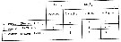
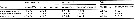
| | | | | | | | | | | | | | | 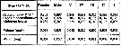 issued from : A.A. Shmeleva in Bull. Inst. Oceanogr., Monaco, 1965, 65 (n°1351). [Table 6: 16 ]. Ctenocalanus vanus (from South Adriatic). issued from : A.A. Shmeleva in Bull. Inst. Oceanogr., Monaco, 1965, 65 (n°1351). [Table 6: 16 ]. Ctenocalanus vanus (from South Adriatic).
Dimensions, volume and Weight wet. Means for 50-60 specimens. Volume and weight calculated by geometrical method. Assumed that the specific gravity of the Copepod body is equal to 1, then the volume will correspond to the weight. |
 issued from : C. de O. Dias & A.V. Araujo in Atlas Zoopl. reg. central da Zona Econ. exclus. brasileira, S.L. Costa Bonecker (Edit), 2006, Série Livros 21. [p.44]. issued from : C. de O. Dias & A.V. Araujo in Atlas Zoopl. reg. central da Zona Econ. exclus. brasileira, S.L. Costa Bonecker (Edit), 2006, Série Livros 21. [p.44].
Chart of occurrence in Brazilian waters (sampling between 22°-23° S)
Nota: sampling only 4 specimens. |
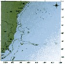
 issued from : U. Brenning in Wiss. Z. Wilhelm-Pieck-Univ. Rostock - 31. Jahrgang 1982 a. Mat.-nat. wiss. Reihe, 6. [p.1, Fig.1]. issued from : U. Brenning in Wiss. Z. Wilhelm-Pieck-Univ. Rostock - 31. Jahrgang 1982 a. Mat.-nat. wiss. Reihe, 6. [p.1, Fig.1].
Spatial distribution for Ctenocalanus vanus from 8° S - 26° N; 16°- 20° W, for expedition V1: Dec. 1972- Jan. 1973. |
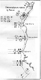
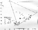
 issued from : U. Brenning in Wiss. Z. Wilhelm-Pieck-Univ. Rostock - 31. Jahrgang 1982 a. Mat.-nat. wiss. Reihe, 6. [p.14, Fig.5]. issued from : U. Brenning in Wiss. Z. Wilhelm-Pieck-Univ. Rostock - 31. Jahrgang 1982 a. Mat.-nat. wiss. Reihe, 6. [p.14, Fig.5].
Spatial distribution for Ctenocalanus vanus from Namibia (SW Africa) for expedition VIII: 21/9- 17/12 1976 . |
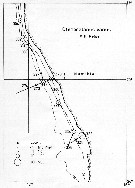
 issued from : U. Brenning in Wiss. Z. Wilhelm-Pieck-Univ. Rostock - 31. Jahrgang 1982 a. Mat.-nat. wiss. Reihe, 6. [p.14, Fig.6]. issued from : U. Brenning in Wiss. Z. Wilhelm-Pieck-Univ. Rostock - 31. Jahrgang 1982 a. Mat.-nat. wiss. Reihe, 6. [p.14, Fig.6].
E-S diagram for Ctenocalanus vanus from 8° S - 26° N; 16°- 20° W (NW Africa) and Namibia (SW Africa), for diferent expeditions (V1: Dec. 1972- Jan. 1973 and VIII: 21/9-17/12 1976).
SO: Southern Surface Water (S °/oo: 34,50; T°C: 29,0); ND: Northern Water of the Surface Layer (S °/oo: 37,5; T°C: 21,0); SD: Southern Deep Water of the surface layer (S °/oo: 35,33; T°C: 13,4). See commentary in Temora stylifera and Brenning (1985 a, p.6). |
 issued from : U. Brenning in Wiss. Z. Wilhelm-Pieck-Univ. Rostock - 31. Jahrgang 1982 a. Mat.-nat. wiss. Reihe, 6. [p.15, Fig.7]. issued from : U. Brenning in Wiss. Z. Wilhelm-Pieck-Univ. Rostock - 31. Jahrgang 1982 a. Mat.-nat. wiss. Reihe, 6. [p.15, Fig.7].
Vertical distribution for Ctenocalanus vanus from 8° S - 26° N; 16°- 20° W, for expedition V1 ( Dec. 1972- Jan. 1973).
T = daylight; N = night; G = total; W = females; CV = copepodid stages 5. |
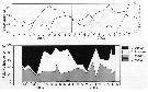 issued from : A. Cornils, B. Niehoff, C. Richter, T. Al-Najjar & B. Schnack-Schiel in J. Plankton Res., 2007, 29 (1). [p.60, Figs.1, 2]. issued from : A. Cornils, B. Niehoff, C. Richter, T. Al-Najjar & B. Schnack-Schiel in J. Plankton Res., 2007, 29 (1). [p.60, Figs.1, 2].
Above: Annual cycle of sea surface temperature and depth -integrated (0-100 m) chlorophyll a (mg/m2)
Below: Relative frequency (%) of the clausocalanid females over the investigation period (March 2002 to December 2003) in the northern Gulf of Aqaba (29°27'87 N, 34°57' 87 E; depth 300 m) for Ctenocalanus vanus and Clausocalanus minor, C. farrani, C. furcatus.
Nota: Collected by vertical hauls from 100 m depth to the surface. Sampling performed between 9 a.m. and 3 p.m. on a monthly basis. |
 issued from : A. Cornils, B. Niehoff, C. Richter, T. Al-Najjar & B. Schnack-Schiel in J. Plankton Res., 2007, 29 (1). [p.65, Fig.8]. issued from : A. Cornils, B. Niehoff, C. Richter, T. Al-Najjar & B. Schnack-Schiel in J. Plankton Res., 2007, 29 (1). [p.65, Fig.8].
Prosome length (mm) displayed with SE bars over the investigation period. |
 issued from : A. Cornils, B. Niehoff, C. Richter, T. Al-Najjar & B. Schnack-Schiel in J. Plankton Res., 2007, 29 (1). [p.65, Table III]. issued from : A. Cornils, B. Niehoff, C. Richter, T. Al-Najjar & B. Schnack-Schiel in J. Plankton Res., 2007, 29 (1). [p.65, Table III].
Percentage of clausocalanid females infected with Blastodinium sp. (dinoflagellate) or showing abnormalities of the P5 (%), found in the preserved females. |
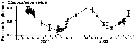
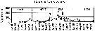 Issued from : W.T. Peterson, J.E. Keister & L.R. Feinberg in Prog. Oceanogr., 2002, 54. [p.393, Fig.8]. Issued from : W.T. Peterson, J.E. Keister & L.R. Feinberg in Prog. Oceanogr., 2002, 54. [p.393, Fig.8].
Abundance (number per cubic meter) of Ctenocalanus vanus at the station NH5 (off Newport, Oregon, at depth 30 m) from May 1996 through September 1999.
Compare with Calanus marshallae and Pseudocalanus mimus at the same station during El Niño event in 1997-98, the largest of the century. |
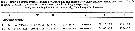 Issued from : M.D. Viñas, N.R. Diovisalvi & G.D. Cepeda in J. Braz. Oceanogr., 2010, 58 (2). [p.178, Table 1]. Issued from : M.D. Viñas, N.R. Diovisalvi & G.D. Cepeda in J. Braz. Oceanogr., 2010, 58 (2). [p.178, Table 1].
Body dimensions and estimated biovolume of Ctenocalanus vanus samples on October 18th and November 11th at the permanent coastal station (38°28'S, 57°41'W).
Body wet weight can be derived from measurements of body volume by applying a factor of 1 for specific gravity. Dry weight can be obtained by mulitplyng the wet weight by 0.20 and the carbon content as 40% of the dry weight.
F: female; M: male.
Prosome length, width and height, as well as urosome length and width, were measured, in order to apply the model of Chojancki & Hussein (1983) slightly modified (antenna and leg volume excluded) by Fernadez Araoz (1991). |
| | | | Loc: | | | [? Antarct. (Peninsula, Atlant. SW, South Georgia, SE, Indian, SW & SE Pacif.)], ? Magallanes region, sub-Antarct. (S Patagonia, off Prince Edward Is., Indian, S Kerguelen Is. SW & SE Pacif.), Benguela Current, South Africa (E & W), Saldanha, Namibia, Angola, Baia Farta, Congo, G. of Guinea, Ivorian shelf, off S Cape Verde Is., Senegal-Mauritania, Morocco-Mauritania, Cap Ghir (Morocco), Canary Is, off Madeira, Patagonia, Peninsula Valdés, Mar del Plata, Uruguay (continental shelf), Brazil (off Rio de Janeiro, Campos Basin, Cabo Frio, off Cabo de Sao Tomé), off Amazon, Caribbean Sea, Caribbean Colombia, Gulf of Mexico, Florida, Sargasso Sea, off Bermuda: Station "S" (32°10'N, 64°30'W), Faroe Is., W Ireland, off SW Ireland, W Enlish Channel (Morlaix estuary), Belon estuary, Bay of Biscay, off Coruña, off W Cape Finisterre, Portugal, Ibero-moroccan Bay, Medit. (Alboran Sea, Habibas Is., Algiers, Gulf of Annaba, Baleares, Banyuls, Marseille, Ligurian Sea, Tyrrhenian Sea, G. of Napoli, Lake Faro, Strait of Messina, Taranto, G. of Trieste, Island of Pag, Adriatic Sea, Ionian Sea, Aegean Sea, Thracian Sea, Alexandria, Lebanon Basin, Marmara Sea, Black Sea), Gulf of Suez, G. of Aqaba, off Sharm El-Sheikh, Safâga, Red Sea, SW Indian (Natal), Madagascar, Indonesia (SW Celebes), Australia (North West Cape), China Seas (Yellow Sea, East China Sea, South China Sea), Taiwan Strait, Taiwan (NW, N, Mienhua Canyon), Korea, Korea Strait, Japan (Honshu: Toyama Bay Suruga Bay, Sagami Bay), Japan Sea, Tsushima Straits, Japan, Tokyo Bay, Suruga Bay, off SE Japan, off Washington coast, Oregon (Yaquina, off Newport), California (Bay of San Francisco, San Diego), W Baja California, Bahia Magdalena, G of California, Australia (Great Barrier, New South Wales, Melbourne), New Caledonia, New Zealand (Kaikoura), off Hawaï N, Chile (N-S, off Valparaiso, off Santiago, Concepcion) | | | | N: | 283 ? (any confusion with Ctenocalanus citer in the South Ocean) | | | | Lg.: | | | (14) F: 1,31-1,1; (22) F: 1,21; M: 1,36; (34) F: 1,1-0,81; M: 1,2; (35) [Atlant. trop.] F: 1,25-1,2; [N-Z] F: 1,2-1,02; (38) F: 1,16-0,92; M: 1,26-1,2; (54) F: 1,03-0,95; M: 1,13; (55) F: 1,27; M: 1,4-1,25; (66) F: 1,27-0,97; M: 1,2-1,1; (72) F: 1,28-1,06; (104) F: 1,36; M: 1,31; (114) F: 1,16; (116) F: 1,02; (128) F: 1,27; (131) F: 1,27-0,95; M: 1,4-1,08; (145) F: 1,21; M: 1,36; (199) F: 1,14-0,99; (202) F:(237) F: 1,5; 1,25-1,1; M: 1,33-1,25; (246) F: 1,15-1,03; (327) F: 1,37-1,01; M: 1,36-1,19; (338) F: 1,05-1,13; M: 1,20-1,28; (373) F: 1,27; (432) F: 1,7-1,2; M: 1,95-1,2; (449) F: 1,1; (786) F: 1,3-1,18; (861) F: 1,25-1,27; M: 1,35-1,36; (1113) F: 0,96-1,25; M: 1,1-1,3 [NW Africa]; F: 0,91-1,44 [SW Africa]; (1185) F: 1,32-1,00: M: 1,37-1,31; {F: 0,81-1,70; M: 1,08-1,95}
The mean female size is 1.163 mm (n = 49; SD = 0.1679) and the mean male size is 1.289 mm (n = 27; SD = 0.1627). The size ratio (male : female) is 1.094 (n = 16; SD = 0.0766).
Chiba S. & al., 2015 (p.971, Table 1: Total length female (June-July) = 1.1 mm [optimal SST (°C) = 14.3]. | | | | Rem.: | épi-bathypélagique (probably mainly 0-200 m).
Sampling depth (sub-Antarct.) : 0-200 m.
Certaines formes antarctiques ou subantactiques peuvent avoir été confondues avec C. citer, comme en d'autres lieux.
Observé dans les ballasts des navires à San Francisco.
C. Séret (1979, p.56) note la présence de cette espèce à 2 stations: 56°S, 70°E et 51°S, 65°E, proche des Îles Kerguelen et la distingue bien de C. citer.
Voir aussi les remarques en anglais | | | Dernière mise à jour : 28/10/2022 | |
|
|
 Toute utilisation de ce site pour une publication sera mentionnée avec la référence suivante : Toute utilisation de ce site pour une publication sera mentionnée avec la référence suivante :
Razouls C., Desreumaux N., Kouwenberg J. et de Bovée F., 2005-2026. - Biodiversité des Copépodes planctoniques marins (morphologie, répartition géographique et données biologiques). Sorbonne Université, CNRS. Disponible sur http://copepodes.obs-banyuls.fr [Accédé le 14 avril 2026] © copyright 2005-2026 Sorbonne Université, CNRS
|
|
|
|


;)
;)
;)
;)
;)
;)
;)
;)
;)
;)
;)
;)
;)
;)
;)
;)
;)
;)
;)
;)

;)
;)
;)
;)
;)
;)