|
|
 |
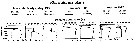
Fiche d'espèce de Copépode |
|
|
Calanoida ( Ordre ) |
|
|
|
Eucalanoidea ( Superfamille ) |
|
|
|
Rhincalanidae ( Famille ) |
|
|
|
Rhincalanus ( Genre ) |
|
|
| |
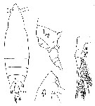
Rhincalanus gigas Brady, 1883 (F,M) | |
| | | | | | | Syn.: | Rhincalanus grandis Giesbrecht, 1902 (p.18, figs.F); Wolfenden, 1908 (p.14, fig.F); 1911 (p.194);
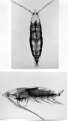
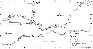
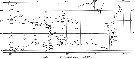
no R. gigas : T. Scott, 1902 (p.450); A. Scott, 1909 (p.24, Rem.); Sewell, 1914 a (p.203) | | | | Ref.: | | | Brady, 1883 (part.: large antractic forms, p.42, figs.F); Giesbrecht & Schmeil, 1898 (p.23); T. Scott, 1912 (1913) (p.530); Brady, 1918 (p.16, figs.F, M, Rem.); Schmaus & Lehnhofer, 1927 (p.361, figs.F,M, Rem.); Sewell, 1929 (p.59-60, Rem.); Farran, 1929 (p.208, 220, Rem.); Mackintosh, 1934 (p.85) ; Steuer, 1935 (p.383, figs.N, , Rem.: copepodites); Gibbons, 1936 (p.383, figs.N); Vervoort, 1946 (p.116); 1951 (p.57, Rem.); 1957 (p.34, Rem.); Tanaka, 1960 (p.21, figs.F, Rem., juv.M); Ramirez, 1969 (p.47, figs.F, juv.M, Rem.); Silas, 1972 (p.645); Séret, 1979 (p.42); Björnberg & al., 1981 (p.621, figs.F,M); Sazhina, 1985 (p.36, figs.N); Prado Por, 1986 (p.517); Razouls, 1994 (p.40, figs.F,M); Bradford-Grieve, 1994 (p.84, figs.F,M, fig.100); Bradford-Grieve & al., 1999 (p.878, 912, figs.F,M); Braga & al., 1999 (p.79, 84, tab.1, Rem.: Biol. mol.); Ferrari & Markhaseva, 2000 (p.84, fig.); Goetze, 2003 (p.2322 & suiv.); Boxshall & Halsey, 2004 (p.176); Michels & Schnack-Schiel, 2005 (p.483, fig.4: Md); Ferrari & Dahms, 2007 (p.62); Stupnikova & al., 2013 (p.451, genetic); Cheng F. & al., 2013 (p.119, molecular biology, GenBank); Xavier & al., 2020 (p.28, fig., Rem.). | 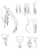 juvenil Female : 1, habitus (lateral); 2, 2', P5; issued from : Brady in Rep. scient. Results Voy. Challenger, Zool., 1883, 8 (23): 1-142. Female: 3, P5; 4, 5, Th5 and Urosome (lateral, dorsal); issued from : Ramirez, 1969. Juvenil Male: 6, P5 (G: left, Dt right). issued from : Ramirez, 1969. Male: 7, P5; issued from : Schmaus & Lehnhofer in Wiss. Ergebn. dt. Tiefsee-Exped. \"Valdivia\", 1927, 23: 355-400.
|
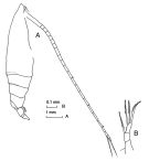 issued from : J.M. Bradford-Grieve in The Marine Fauna of New Zealand: Pelagic Calanoid Copepoda. National Institute of Water and Atmospheric Research (NIWA). New Zealand Oceanographic Institute Memoir, 102, 1994. [p.84, Fig.45]. Female: A, habitus lateral right side); B, P5.
|
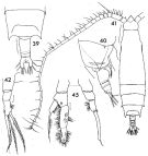 issued from : F.C. Ramirez in Contr. Inst. Biol. mar., Buenos Aires, 1969, 98. [p.46, Lam. VII, figs.39, 40, 41, 42, 45 ]. Female (from off Mar del Plata): 39, posterior part of prosome and urosome (dorsal); 40, idem (lateral right side); 42, P5. Juvenil male: 41, habitus (dorsal); 45, P5. Scale bars in mm: 0.2 (39, 40); 0.05 (42, 45); 1 (41).
|
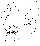
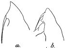 issued from : R.B.S. Sewell in Mem. Indian Mus., 1929, X. [p.59, Fig.19]. a, forehead (lateral; from off SE Sri Lanka); b, forehead in (from South Ocean)
|
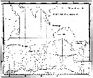
 issued from : R.B.S. Sewell in Mem. Indian Mus., 1929, X. [p.60]. Main points of difference between R. gigas and R. nasutus.
|
 issued from : J. Michels & S.B. Schnack-Schiel in Mar. Biol., 2005, 146. [p.487, Fig.4]. Mandibular gnathobase. a, Female (from Weddell and Bellingshausen Seas); b, Male. a, b: left gnathobase from cranial; V: ventral tooth, C1-C4: central teeth, D1-D3: dorsal teeth, B: dorsal bristle; R: ridge-like-structure; arrow: the cone-shaped structure. Scale bars 0.020 mm.
|
 issued from : W. Giesbrecht in Copepoden. Res. voyage du S. Y. Belgica. Rapports scientifiques, Zoologie, 1902. [Taf. I, Figs.15-18]. As Rhincalanus grandis. Female (from S, SE Peter Ist Island)): 15, habitus (dorsal); 16, forehead (lateral); 17, posterior part of prosome and urosome (lateral); 18, P5.
|
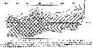
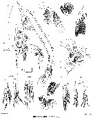 Issued from : G.S. Brady in Rep. Scient. Results Voy. Challenger, Zool., 1883, 8 (23). [Pl.VIII]. Female: 1, habitus (lateral); 1a, last thopracic segment (seen from below); 2, A2; 3, Md; 4, mx1; 5, mx2; 6, Mxp; 7, P1; 8, P4; 9, P5; 10, P5 from another specimen; 11, urosome. Nota; See below remarks from Vervoort
|
 issued from : C. Razouls (pers. coll.). Female (dorsal and lateral) from Kerguelen Islands, 21 October 1995.
|
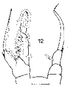
 Issued from : J.M. Bradford in N.Z. Oceanogr. Inst., 1971, 206, Part 8, No 59. [p.15, Figs.13, 14]. Female (from Ross Sea):13-14, P5. Scale bar: 100 µm.
|
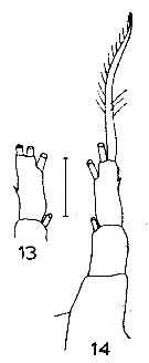
 Issued from : J.M. Bradford in N.Z. Oceanogr. Inst., 1971, 206, Part 8, No 59. [p.15, Fig.12]. Male (from Ross Sea): 12, P5. Scale bar: 100 µm.
|
 Issued from : O. Tanaka in Spec. Publs. Seto mar. biol. Lab., 10, 1960 [Pl. V]. Female (from 66°59'S-67°03'S, 41°08'E-40°44'E): 1, head (lateral); 2, same (ventral); 3, last thoracic segment and urosome (lateral). Nota: Cephalothorax and abdomen in the proportional lengths 86 to 14. Frontal margin of the head produced. Rostral filaments slender and long. 3re and 4th thoracic segments furnished with a lateral spine on each side. Abdomen 3-segmented. The anal segment fused with the caudal rami. Abdominal segments and caudal rami in the proportional lengths 46 : 12 : 21 : 21 = 100. Genital segment produced ventrally. P5 small and 3-segmented; the distal segment carries 3 apical and 1 marginal setae.
|
 Issued from : C. Razouls in Ann. Inst. océanogr., Paris, 1994, 70 (1). [p.40]. Caractéristiques morphologiques de Rhincalanus gigas femelle et mâle adultes. Terminologie et abbréviations: voir à Calanus propinquus.
| | | | | Ref. compl.: | | | Hardy & Gunther, 1935 (1936) (p.140, distribution charts); Ottestad, 1936 (p.11, 21, 26, 35, vertical and antarctic distribution); Ommanney, 1936 (p.277, seasonal vertical migrations); Baker, 1954 (p.203, 211, fig.5); Brodsky, 1964 (p.105, Rem.: p.109); Murano, 1965 (p.91, fig.4, abundance, geographic distribution); Grice & Hulsemann, 1967 (p.14); Vinogradov, 1968 (1970) (p.66, 67, 234); Voronina, 1970 (p.162, spatial & vertical distributions); 1972 (p.336, vertical distribution); 1972 a (p.415, vertical distribution); Björnberg, 1973 (p.297, 388); Rakuza-Suszczewski & al., 1976 (p.763, respiration); Voronina & Sukhanova, 1976 (1977) (p.614, food composition); Vladimirskaya, 1978 (p.202, vertical distribution, age composition); Voronina & al., 1978 (p.512, distribution); 1980 a (p.1079, annual cycle, production); Biggs, 1982 (p.55, Table 2: NH4 excretion, O2 consumption); De Decker, 1984 (p.315); Hubold, 1985 (p.43, Table 1, predation by fish); Bamstedt & Tande, 1985 (p.259, Table 2: literature data respiration & excretion); Hopkins, 1985 (p.197, Table 1, gut contents); Dearborn & al., 1986 (p.1, predation by benthic star); Reinhardt & Van Vleet, 1986 (p.149, lipid composition); Zmijewska, 1987 (tab.2a); Hopkins & Torres, 1988 (tab.1); Ferrari & Dearborn, 1989 (p.1319); Ward, 1989 (tab.2); Ferrari & Dearborn, 1989 (p.1315, predation); Perissinotto, 1989 (p.505, Table 2, 3, abundance, diurnal variation); Trofimov & al., 1989 (p.426); Atkinson & al., 1990 (p.1213, tab.1); Øresland, 1990 (p.201, Table 1, predator); Atkinson, 1991 (p.79, antarctic zonation, seasonal change, vertical distribution, life history); Conover & Huntley, 1991 (p.1, Table 2, 3, 5, 7, 9, 10, 13, polar seas comparison); Rau & al., 1991 (p.1, isotopic forms vs feeding); Atkinson & al., 1992 (p.583, diel vertical migration, feeding); 1992 a (p.49, feeding rates, vertical migration); Siegel & al., 1992 (p.18, tab.3,4); Huntley & Lopez, 1992 (p.201, Table A1, B1, egg-adult weight, temperature-dependent production, growth rate); Perissinotto & McQuaid, 1992 (p.15, predation v.s. migration); Freire & al., 1993 (tab.3); Marin & Schnack-Schiel, 1993 (p.35, vertical distribution); Zmijewska, 1993 (p.73, seasonal and spatial variations); Bathmann & al., 1993 (p.333, chart distribution); Jiyalal Ram & Goswami, 1993 (p.129, tab.IV); Hosie & Cochran, 1994 (p.21, tab.1, 2, fig.2, 9); Schnack-Schiel & Hagen, 1994 (p.1543, life cycle); Atkinson, 1994 (p.551, feeding selectivity); 1994 a (p.1, feeding); Graeve & al., 1994 (p.915, lipid composition v.s. diet); Kattner & al., 1994 (p.637, lipid seasonal changes); Donnelly & al., 1994 (p.171, chemical composition); Ward & al., 1995 (p.195, abundance, biomass, vertical distribution); Ward & Shreeve, 1995 (p.721, egg production); Atkinson & Shreeve, 1995 (p.1291, feeding activity); Atkinson & al., 1996 (p.195, feeding vs. phytoplankton bloom); Atkinson & al., 1996 (p.1387, diel periodicity, feeding); Ward & al., 1996 (p.21, distribution and dynamic population); Ward & al., 1996 (p.1439, lipid storage); Hagen & Schnack-Schiel, 1996 (p.139, seasonal lipid, maturity); Pakhomov & McQuaid, 1996 (p.271, abundance, distribution, seabirds); Froneman & al., 1996 (p.15, nutrition, grazing); Froneman & al., 1997 (p.201, abundance, grazing); Zmijewska & al., 1997 (p.127); Errhif & al., 1997 (p.422); Ward & al., 1997 (p.261); Vuorinen & al., 1997 (p.280); Beaumont & Hosie, 1997 (p.121, spatial distribution); Fransz & Gonzalez, 1997 (p.395, weight-length, biomass vs. N-S transect); Spiridonov & Kosobokova, 1997 (p.233, spatial distribution, vertical migration); Elwers & Dahms, 1998 (p151); Voronina, 1998 (p.375, biomass); Mauchline, 1998 (tab.21, 27, 30, 33, 38, 45, 58); Ward & Shreeve, 1998 (p.142, fig.1, egg hatching vs temperature); Atkinson, 1998 (p.289, Table 1, biological data); Atkinson & al., 1999 (p.63, Krill-copepod interactions, fig.6, 7: diel migration); Tirelli & Mayzaud, 1999 (p.197, gut evacuation); Atkinson & Sinclair, 2000 (p.46, 50, 51, 53, 55, zonal distribution); Razouls & al., 2000 (p.343, tab. 5, Appendix); Pakhomov & al., 2000 (p.1663, Table 1, 2, transect Cape Town-SANAE antarctic base); Chiba & al., 2001 (p.95, tab.4, 7); Pasternak & Schnack-Schiel, 2001 (p.25); Voronina & al., 2001 (p.401); Li & al., 2001 (p.894, tab.1); Hunt & al., 2001 (p.374, tab.1, 2); Voronina, 2002 (p.68, abundance vs stations); Cabal & al., 2002 (p.869, fig.4, Table 1, abundance); Ward & al., 2002 (p.2183, tab.2, 3, fig.7); Takahashi & al., 2002 (p.97, Table 2, fig.5); Ward & al., 2003 (p.121, tab.4); Kahle & Zauke, 2003 (p.409, metals concentration); Hunt, 2004 (p.1, 43, 74, Table 3.2, 4.4, fig.4.7, 4.11, Rem.: p.94, fig.5.10: seasonal abundance); Calbet & al., 2005 (p.1195, tab.3); Ward & al., 2005 (p.421, Table 6, 8, 9, nauplii abundance, biomass, egg production); Ward & al., 2006 (p.83: tab.4); Hunt & Hosie, 2006 (p.1182, seasonal succession, indicator); 2006 a (p.1203, tab.2,fig.8); Schultes & al., 2006 (p.16, fig.1); Tsujimoto & al., 2006 (p.140, Table1); Deibel & Daly, 2007 (p.271, Table 6a, 6b, 7a, Rem.: Antarctic polynyas); Fielding & al., 2007 (p.2106, tab.1); Khelifi-Touhami & al., 2007 (p.327, Table 1); Ward & al., 2007 (p.1871, Table 2, fig.6, 7, abundance, egg production); Kattner & al., 2007 (p.1628, Table 1); Schnack-Schiel & al., 2008 (p.1045: Tab.2); Ward & al., 2008 (p.241, Tabls, Appendix II ); Klaas & al., 2008 (p.195, fig.2, grazing); Kruse & al., 2009 (p.301, gut content); Park & Ferrari, 2009 (p.143, Table 2, fig.1, Appendix 1, biogeography); Takahashi & al., 2010 (p.317, Table 3, 4, fig.5); Goetze & Ohman, 2010 (p.2110, Table 1); Sartoris & al., 2010 (p.1860, buoyancy, diapause, hemolymph cation concentration); Takahashi & al., 2010 (p.235, Table 2); Swadling & al., 2010 (p.887, Table 2, 3, A1, fig.6, abundance, indicator species); Hsiao & al., 2010 (p.179, Table III, trace metal concentration); Yang & al., 2011 (p.1065, fig.2d); Yang & al., 2011 a (p.921, Table 2, inter-annual variation 1999-2006); 2011 a (p.1614, Table 2, Fig.2A, 5, 6); 2011 a (p.1614, Table 2, Fig.2A, 5, 6); Takahashi & al., 2011 (p.134, distribution); Swadling & al., 2011 (p.118, Table 2, figs. 5, 7, interannual abundance); Tutasi & al., 2011 (p.791, Table 2, abundance distribution vs La Niña event); Ward & al., 2012 (p.78, Table 1, fig.5, 6, Table A1, B1, C1, abundance, weight, depth); Thompson G.A. & al., 2012 (p.127, Table 2, 3); Thompson G. & al., 2012 (p.367, Rem.: p.376); Michels & al., 2012 (p.369, Table 1, occurrence frequency); Tarling & al., 2012 (p.222, Table 1, 3, seasonal biomass); Mackey & al., 2012 (p.130, Table 1, 2, Fig.2, abundance, climate change projections); Yang G. & al., 2013 (p.1701, fig.4, Table 2, feeding); Schründer & al., 2013 (p.1, sodium/ammonium and ph effects in the hemolymph); Ojima & al., 2013 (p.1293, Table 2, 3, abundance); Lee D.B. & al., 2013 (p.1215, Table 1, 2, 3, 4, abundance, composition, grazing, C ration); Ward & al., 2014 (p.305, Table 4, abundance in the ''Discovery'' Investigations in the 1930s); Record & al., 2018 (p.2238, Table 1: diapause); Acha & al., 2020 (p.1, Table 3: occurrence % vs ecoregions). | | | | NZ: | 7 + 1 douteuse | | |
|
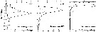
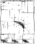
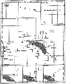
Carte de distribution de Rhincalanus gigas par zones géographiques
|
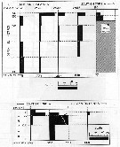
| | | | | | | | | | | | 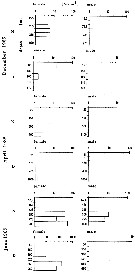 Issued from : M.I. Zmijewska in Oceanologia, 1993, 35. [Fig. 3.3]. Issued from : M.I. Zmijewska in Oceanologia, 1993, 35. [Fig. 3.3].
Diel changes in abundance distribution (ind./ m2) of Rhincalanus gigas adult female and male (from 64°50'S, 61°50'W, Croker Passage, Antarctic Peninsula) during 3 austral seasons.
N = night; D = day. |
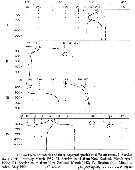
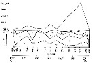
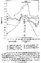
 Issued from : A. Atkinson in Mar. Biol., 1991, 109. [p.82, Fig.2] Issued from : A. Atkinson in Mar. Biol., 1991, 109. [p.82, Fig.2]
Rhincalanus gigas. Mean abundance (nos./1000 m) of vertical haul) in top 1 000 m within five water types. bars represent standard errors of means, calculated from assumed Poisson distribution.
Estimated contributions to total copepod biomass in study area: 36 % %.
Nota: Water types:
1- Either in sub-Antarctic zone or in vicinity of subantarctic front.
2- Within polar frontal zone.
3- In vicinity of polar front.
4- Within Antarctic zone.
5- Within Weddell Sea or in Weddell-Scotia confluence. |
 Issued from : A. Atkinson in Mar. Biol., 1991, 109. [p.80, Fig.1]. Issued from : A. Atkinson in Mar. Biol., 1991, 109. [p.80, Fig.1].
Positions of 72 stations sampled in Scotia Sea. The Scotia Sea, containing majority of stations, is bordered on east by a chain of oceanic islands and on west by Drake Passage (between South America and the Antarctic Peninsula.
Mean positions of oceanic fronts, and zones which they separate are drawn from Gordon (1967).
SAF: subantarctic front.
PFZ: polar frontal zone.
PF: polar front.
AZ: Antarctic zone.
WSC: Weddell-Scotia confluence. |
 Issued from : A. Atkinson in Mar. Biol., 1991, 109. [p.82, Fig.3]. Issued from : A. Atkinson in Mar. Biol., 1991, 109. [p.82, Fig.3].
Rhincalanus gigas. Mean vertical distribution during four seasons. Values are numbers/250 m of vertical haul. |
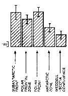
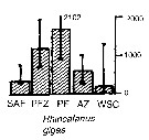 Issued from : A. Atkinson & J.D. Sinclair in Polar Biol., 2000, 23. [p.50, Fig.3] Issued from : A. Atkinson & J.D. Sinclair in Polar Biol., 2000, 23. [p.50, Fig.3]
Rhincalanus gigas from Scotia Sea.
Median and interquartile ranges of copepods (nos /m2) in the five water zones; from north to south these are SAF Subantractic Front area, PFZ Polar frontal Zone, PF Polar Front area, AZ Antarctic Zone, WSC Weddell-Scotia Confluence area/ East Wind Drift.
Numbers on the plots are upper interquartiles where these could not be scaled. |
 Issued from : V.A. Spiridonov & K.N. Kosobokova in Mar. Ecol. Prog. Ser., 1997, 157. [p.236, Fig.2 (modified)]. Issued from : V.A. Spiridonov & K.N. Kosobokova in Mar. Ecol. Prog. Ser., 1997, 157. [p.236, Fig.2 (modified)].
Abundance of Calanoides acutus, Calanus propinquus and Rhincalanus giga (A) along the Greenwich transect in the upper 0 to 500 m water layer from subantarctic to Antarctic continent (stations 571 to 606), in early to mid-winter.
PF: Polar front; ACC: Antarctic Circumpolar Current; WF: Weddell Front; MR: Maud Rise; CWB: Continental Water Boundary. |
 Issued from : V.A. Spiridonov & K.N. Kosobokova in Mar. Ecol. Prog. Ser., 1997, 157. [p.239, Fig.9]. Issued from : V.A. Spiridonov & K.N. Kosobokova in Mar. Ecol. Prog. Ser., 1997, 157. [p.239, Fig.9].
Vertical distribution of temperature (°C) and characteristics of the vertical distribution of particular copepodite stages of Rhincalanus gigas sampled from surface to 1000 m depth along the Greenwich transect from 55°S (station 576) to 69°S (station 603).
Vertical lines (1) show the range of occurrence, horizontal bars (2) mark the median depth of occurrence, and rectangles (3) cover the range centered around the median depth where a core (50% of a hemipopulation) is concentrated.
C1 to C6: copepodite stages. |
 Issued from : S.B. Schnack-Schiel & W. Hagen in J. Plankton Res., 1994, 16 (11). [p.1553, Fig.9]. Issued from : S.B. Schnack-Schiel & W. Hagen in J. Plankton Res., 1994, 16 (11). [p.1553, Fig.9].
Vertical distribution of R. gigas from eastern Weddell Sea, as a percent of total numbers and temperature profile within the upper 1000 m. |
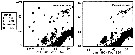
 Issued from : M. Murano inThe Ocean Res. Inst., Univ. Tokyo, 1965. Coll. Rep., 1964, Vol.3. [p.103, Fig.4]. Issued from : M. Murano inThe Ocean Res. Inst., Univ. Tokyo, 1965. Coll. Rep., 1964, Vol.3. [p.103, Fig.4].
The quantitative distribution of Rhincalanus gigas Brady, gathered by NORPAC net, hauls vertically up to the water surface from a depth of 200 m between December, 1961 and February, 1962. |
 issued from A. de C. Baker in 'Discovery' Rep., 1954, 27. [p.215, Fig.5]. issued from A. de C. Baker in 'Discovery' Rep., 1954, 27. [p.215, Fig.5].
Occurrence of Rhincalanus gigas in all longitudes around Antarctic zone of the Southern Ocean.
The percentage frequency of occurrence in samples taken within every 20° of longitude.
Nota: During the 'Discovery' investigations some thousands of plankton samples have been taken from stations spread over the whole of the Southern Ocean at all seasons of the year, the majority south of the Antarctic Convergence. An arbitrary selection of samples has been made from hauls between the surface and a depth of 250 m, which means that they have been taken from within the limits of the Antarctic surface water.
The data suggest that the Southern Ocean is an uninterrupted circumpolar belt with more or less uniform conditions prevailing in east and west directions, the range of planktonic species of the Antarctic surface water may be expected to extend as far as these uniform conditions persist, i.e to be circumpolar. |
 Issued from : P. Ward, A. Atkinson, A.W.A. Murray, A.G. Wood, R. Williams & S. Poulet in Polar Biol., 1995, 15. [p.200, Fig.3]. Issued from : P. Ward, A. Atkinson, A.W.A. Murray, A.G. Wood, R. Williams & S. Poulet in Polar Biol., 1995, 15. [p.200, Fig.3].
Abundance and biomass (g dry mass/m3) profiles for the shelf station (54°48'S, 38°15'W) in January 1990.
Values on the horizontal axes at the base represent abundance and the one above biomass. Solid line = midday haul; hatched line = midnight haul. |
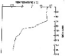 Issued from : P. Ward, A. Atkinson, A.W.A. Murray, A.G. Wood, R. Williams & S. Poulet in Polar Biol., 1995, 15. [p.198, Fig.1, A (modified C.R.)]. Issued from : P. Ward, A. Atkinson, A.W.A. Murray, A.G. Wood, R. Williams & S. Poulet in Polar Biol., 1995, 15. [p.198, Fig.1, A (modified C.R.)].
Temperature profile for the shelf station at Bird Island, South Georgia (54°48'S, 38°15'W) in January 1990. |
 Issued from : P. Ward, A. Atkinson, A.W.A. Murray, A.G. Wood, R. Williams & S. Poulet in Polar Biol., 1995, 15. [p.202, Fig.4, A]. Issued from : P. Ward, A. Atkinson, A.W.A. Murray, A.G. Wood, R. Williams & S. Poulet in Polar Biol., 1995, 15. [p.202, Fig.4, A].
Abundance (10/m3) and biomass (g dry mass/m3) profiles at the oceanic station from the shelf break in water 4000 m deep off Bird Island, South Georgia (53°04'S, 39°51'W) in January 1990.
Values on the horizontal axes at the base of each profile represent abundance and the one above biomass. Solid line = midday haul; hatched line = midnight haul. |
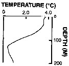 Issued from : P. Ward, A. Atkinson, A.W.A. Murray, A.G. Wood, R. Williams & S. Poulet in Polar Biol., 1995, 15. [p.198, Fig.1, B (modified C.R.)]. Issued from : P. Ward, A. Atkinson, A.W.A. Murray, A.G. Wood, R. Williams & S. Poulet in Polar Biol., 1995, 15. [p.198, Fig.1, B (modified C.R.)].
Profile temperature-depth at the oceanic stations from the shelf break in water 4000 m deep off Bird Island, South Georgia, in January 1990. |
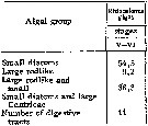 Issued from : N.M. Voronina & I.N. Sukhanova in Oceanology, 1977, 16 (6). [p.615]. Issued from : N.M. Voronina & I.N. Sukhanova in Oceanology, 1977, 16 (6). [p.615].
Frequency of encounter of various groups of diatom algae in the character of leading objects in the food pellet (% of number of digestive tracts with food).
Data from stations between 57°S-69°43'S.
The animals utilize all diatom species from 5 to 300 µm in size, the only animal food found there were tintinnids and radiolarians in negligible quantity. |
 Issued from : N.M. Voronina in Antarctic Ecology, M.W. Holdgate (edit.), 1970, I. [p.170, Fig.7]. Issued from : N.M. Voronina in Antarctic Ecology, M.W. Holdgate (edit.), 1970, I. [p.170, Fig.7].
The northern boundaries of distribution of three copepod species in the 500-0 m layer in the second part of the summer. |
 Issued from : N.M. Voronina in Antarctic Ecology, M.W. Holdgate (edit.), 1970, I. [p.169, Fig.6]. Issued from : N.M. Voronina in Antarctic Ecology, M.W. Holdgate (edit.), 1970, I. [p.169, Fig.6].
The northern boundaries of distribution of three copepod species in the 500-0 m layer at different times. |
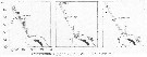
 Issued from : A.C. Hardy & E.R. Gunther in Discovery Reports, 1935 (1936), 11. [p.142, Fig.66]. Issued from : A.C. Hardy & E.R. Gunther in Discovery Reports, 1935 (1936), 11. [p.142, Fig.66].
Charts showing the distribution of Rhincalanus gigas in the upper layers of waters at stations in the 1926-7 surveys around South Georgia.
The squares represent the average numbers per 50 m vertical haul from 250 m (or less at shallow-water stations) to the surface with N 70 V nets.
Compare this Fig.66 with Fig .67 obtained with two nets types (from different mesh apertutres). |
 Issued from : A.C. Hardy & E.R. Gunther in Discovery Reports, 1935 (1936), 11. [p.143, Fig.67]. Issued from : A.C. Hardy & E.R. Gunther in Discovery Reports, 1935 (1936), 11. [p.143, Fig.67].
Charts showing the distribution of Rhincalanus gigas in the upper layers of waters at stations in the 1926-7 surveys around South Georgia.
The squares represent the average numbers per 50 m vertical haul from 250 m (or less at shallow-water stations) to the surface with N 100 H nets.
Compare this Fig.67 with Fig .66 obtained with two nets types (from different mesh apertutres).
Nota: We see that this large copepod was taken in large numbers by the N 100 H nets, which being of a wider mesh than the N 70 V nets let through nearly all yje other copepods (except notably Paraeuchaeta antarctica and Calanus propinquus). They formed quite a prominent feature of these N 100 H samples, along with the Euphausiacea, Amphipoda and other members of the macroplankton. |
 Issued from : E.T. Park & F.D. Ferrari in A selection from Smithsonian at the Poles Contributions to International Polar year. I. Krupnik, M.A. Lang and S.E. Miller, eds., Publs. by Smithsonian Institution Scholarly Press, Washington DC., 2009. [p.165, Fig.1] Issued from : E.T. Park & F.D. Ferrari in A selection from Smithsonian at the Poles Contributions to International Polar year. I. Krupnik, M.A. Lang and S.E. Miller, eds., Publs. by Smithsonian Institution Scholarly Press, Washington DC., 2009. [p.165, Fig.1]
Distribution of selected pelagic calanoids Rhincalanus gigas of the Southern Ocean and the closest relative. |
 Issued from : N.M. Voronina in Oceanology, 2002, 42 (1). [p.71, Fig.3]. Issued from : N.M. Voronina in Oceanology, 2002, 42 (1). [p.71, Fig.3].
Variation in the abundance and age structure (copepodite stages in Roman numerals) of Rhincalanus gigas population along the Antarctic transect at 67°S, within the 0 to 1500 m layer. |
 Issued from : N.M. Voronina in Oceanology, 2002, 42 (1). [p.69, Fig.1]. Issued from : N.M. Voronina in Oceanology, 2002, 42 (1). [p.69, Fig.1].
Hydrological characteristics at the transect from Adelaide Island (Antarctic Peninsula) to the Balleny Island along 67°S during the period from February 23 to March 30, 1992.
Over the greater part of the transect, the vertical temperature distribution was typical of the summer season.
The area studied was located entirely within the waters of the Antarctic vertical structure and covered four segments: The low-latitude ACPC waters (stations 694-733), the high-latitude ACC waters (stations 775, 791 and 793), the mixed waters of both types within the Ross Sea (stations 746-771 and 788), and the shelf waters represented by only a single station on its slope (station 779).
The boundary between the low-latitude and mixed waters of the high latitude modification runs along the pronounced secondary frontal zone in the area of station 739, whereas that between the mixed and properly high-latitude water modifications runs near station 778 (see in Maslennikov, 1992). |
 Issued from : N.M. Voronina in Oceanology, 2002, 42 (1). [p.71]. Issued from : N.M. Voronina in Oceanology, 2002, 42 (1). [p.71].
Average abundance (and its error) of the mass population within different waters (ind./m2 within the 0 to 1500 m layer), n: number of stations. |
 Issued from : J.A. Cabal & al. inDeep-Sea Res., 2002, 49. [p.876, Fig.4]. Issued from : J.A. Cabal & al. inDeep-Sea Res., 2002, 49. [p.876, Fig.4].
Spatial distribution of Rhincalanus gigas in the Northwest Antarctic Peninsula.
Nota: Geographical distribution of stations groups defined by cluster analysis included in the Antarctic Circumpolar Current area and in the coastal waters of the Peninsula, Bransfield and Gerlache Straits during the ''FRUELA'' cruises (December 1995 - February 1996).
Zoopklankton collected by WP2 net from 200-0 m. |
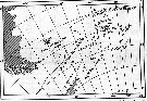
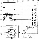
 Issued from : C. Séret in Thesis 3ème Cycle, UPMC, Paris 6. 1979, Annexe. [p.24]. Issued from : C. Séret in Thesis 3ème Cycle, UPMC, Paris 6. 1979, Annexe. [p.24].
Geographical occurrences of Rhincalanus gigas in the Indian Ocean and Antarctic zone. [after publications from: Brady, 1883, 1918; Thompson, 1900; Wolfenden, 1908, 1911; With , 1915; Rosendorn, 1917; Farran, 1929; Sewell, 1929, 1947; Brady & Gunther, 1935; Steuer, 1929, 1392, 1933; Ommaney, 1936; Vervoort, 1957; Tanaka, 1960; Brodsky, 1964; Seno, 1966; Andrews, 1966; Grice & Hulsemann, 1967; Seno, 1966; Frost & Fleminger, 1968; Voronina, 1970; Zverva, 1972]. |
 Issued from : A.C. Hardy & E.R. Gunther in Discovery Reports, 1935 (1936), 11. [p.146, Fig.69]. Issued from : A.C. Hardy & E.R. Gunther in Discovery Reports, 1935 (1936), 11. [p.146, Fig.69].
Vertical distribution of Rhincalanus gigas at stations between the Falkland Islands and South Georgia February 1927 and between South Georgia and Tristan da Cunha February 1926.
The scale represents the numbers per 50 m vertical haul taken by a series of closing N 70 V nets.
Horizontal broken lines show the ranges of these vertical hauls. |
 Issued from : A.C. Hardy & E.R. Gunther in Discovery Reports, 1935 (1936), 11. [p.7, Fig.4]. Issued from : A.C. Hardy & E.R. Gunther in Discovery Reports, 1935 (1936), 11. [p.7, Fig.4].
Chart showing the line of the Antarctic Convergence, separating the Antarctic and the sub-Antarctic Zones, and the course of the two surface currents with influence South Georgia within the Antartic Zone. |
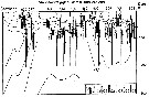
 Issued from : P. Ottestad in On Antarctic Copepods from the ''Norvegia'' Expedition 1930-1931. Scient. Results Norw. Antarct. Exped., 1936, 15. [p.20, Table 10]. Issued from : P. Ottestad in On Antarctic Copepods from the ''Norvegia'' Expedition 1930-1931. Scient. Results Norw. Antarct. Exped., 1936, 15. [p.20, Table 10].
I +II+ III = copepodid stages; depth in meters. Vertical hauls with standard plankton net (Rustad, 1930). |
 Issued from : P. Ottestad in On Antarctic Copepods from the ''Norvegia'' Expedition 1930-1931.Scient. Results Norw. Antarct. Exped., 1936, 15. [ p.19, Table 9]. Issued from : P. Ottestad in On Antarctic Copepods from the ''Norvegia'' Expedition 1930-1931.Scient. Results Norw. Antarct. Exped., 1936, 15. [ p.19, Table 9].
IV, V, VI = copepodid stages; depth in meters. Vertical hauls with standard plankton net (Rustad, 1930). |
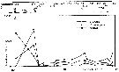
 Issued from : P. Ottestad in On Antarctic Copepods from the ''Norvegia'' Expedition 1930-1931.Scient. Results Norw. Antarct. Exped., 1936, 15. [p.7, Fig.1]. Issued from : P. Ottestad in On Antarctic Copepods from the ''Norvegia'' Expedition 1930-1931.Scient. Results Norw. Antarct. Exped., 1936, 15. [p.7, Fig.1].
The position of the biological stations of ''Norvegica'' 1930-1931. |
 Issued from : K.M. Swadling, F. Penot, C. Vallet & al. in Polar Sci., 2011, 5. [p.125, Fig.5]. Issued from : K.M. Swadling, F. Penot, C. Vallet & al. in Polar Sci., 2011, 5. [p.125, Fig.5].
mean abundance (ind. per 1000 m3) and standard errors of Rhincalanus gigas collected each summer (January), 2004-2008 in the region covered the area from 139°E to 145°E from Terre Adélie to the Mertz Glacier Tongue.
Nota: The entire region sampled during 2004 to 2008 surveys was south of the continental slope and was under the influence of the westward flowing Antarctic Coastal Current. Macrozooplankton were collected by oblique tows of a Bongo net (500 µm mesh aperture) |
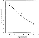 Issued from : P. Ward & R. Shreeve in Polar Biol., 1998, 19. [p.143, Fig.1]. Issued from : P. Ward & R. Shreeve in Polar Biol., 1998, 19. [p.143, Fig.1].
Time to 50% hatching versus temperature (Belehradek function relating embryonic duration; D : days; a = 1305; alpha = - 1120; b fixed as - 2.05) to temperature (T°C) fitted to the data for Rhincalanus gigas from South Georgia (53.5° S, 37° W).
Prosome length = 7.02 mm (± 0.42); egg diameter (outer membrane : 200 µm (± 5). |
 Issued from : V.A. Spiridonov & K.N. Kosobokova in Mar. Ecol. Prog. Ser., 1997, 157. [p.243, Fig.9]. Issued from : V.A. Spiridonov & K.N. Kosobokova in Mar. Ecol. Prog. Ser., 1997, 157. [p.243, Fig.9].
Vertical distribution of temperature (°C) and characteristics of the vertical distribution of copepodite stages (C1 to C6) of Rhincalanus gigas sampled to 1000 m depth at the Greenwhich transect.
Vetical lines (1) show the range of occurrence, horizontal bars (2) mark the median depth of occurrence, and rectangles §3) cover the range centered around the median depth where a core (50% of a hemi-population) is concentrated. |
 Issued from : V.A. Spiridonov & K.N. Kosobokova in Mar. Ecol. Prog. Ser., 1997, 157. [p.234, Fig.1]. Issued from : V.A. Spiridonov & K.N. Kosobokova in Mar. Ecol. Prog. Ser., 1997, 157. [p.234, Fig.1].
Stations at which zooplankton sampling was performed in the Weddell Sea and adjacent areas during the Winter Weddell Gyre Study 1992 (in June-July 1992) |
 Issued from : V.A. Spiridonov & K.N. Kosobokova in Mar. Ecol. Prog. Ser., 1997, 157. [p.236, Fig.2, A]. Issued from : V.A. Spiridonov & K.N. Kosobokova in Mar. Ecol. Prog. Ser., 1997, 157. [p.236, Fig.2, A].
Abundance of Rhincalanus gigas and Calanoides acutus, Calanus propinquus populations along the Greenwich transect in the upper 0 to 500 m water layer. PF: Polar frint; ACC: Antarctic Circumpolar Current; WF: Weddell Fronf; MR: Maud Rise; CWB: Continental Water Boundary. |
 Issued from : A. Atkinson, P. Warde, A. Hill, A.S. Brierley & G.C. Cripps inMar. Ecol. Prog. Ser., 1999, 176. [p.68, Fig.1 (part.)]. Issued from : A. Atkinson, P. Warde, A. Hill, A.S. Brierley & G.C. Cripps inMar. Ecol. Prog. Ser., 1999, 176. [p.68, Fig.1 (part.)].
Abundance of Rhincalanus gigas during Janan-Feb 1994 (low krill biomass), Janv. 1996 (high krill biomass and Dec 1996-Janv 1997 (high krill biomass) figures the right to left, respectively. Shaded bars hauls in feb 1994.
The position of the Polar Front (PF) during each transect is indicated.
Error bars: range in abundance between repeated hauls at a site.
The interaction between copepods and krill (Euphausia superba) is investigated. During two summers of high krill abundance near South Georgia (1996 and 1997) copepod abundance was < 40% of that during an abnormally low krill year (1994). No such depletion was found north of the Polar Front, where krill were rare. An area of persistently high krill abundance just north South Georgia was characterised by exceptionally few copepods. The inverse relationship between krill and copepod abundances thus occurred repeatedly and across a wide range of scales.
The facts that krill swarms are mobile and were unrelated to hydrography further suggest that the inverse relationship was caused by krill. This could arise from competitive exclusion, direct predation or both. Predation is suggested by the fact that crustaceans were found in krill guts in this region during both summer and winter. |
 Issued from : A. Atkinson, P. Warde, A. Hill, A.S. Brierley & G.C. Cripps inMar. Ecol. Prog. Ser., 1999, 176. [p.75, Fig.7]. Issued from : A. Atkinson, P. Warde, A. Hill, A.S. Brierley & G.C. Cripps inMar. Ecol. Prog. Ser., 1999, 176. [p.75, Fig.7].
Median depths of Rhincalanus gigas (CV and CVI females) and other major copepods during a diel series of the Longhurst Hardy Plankton Recorder net (LHPR), profiles in early January 1990.
Nota: Copepods appeared to live deeper and to make more extensive vertical migrations when krill were present |
 Issued from : K.M. Swadling, So. Kawaguchi & G.W. Hosie in Deep-Sea Research II, 2010, 57. [p.898, Fig.6 (continued)]. Issued from : K.M. Swadling, So. Kawaguchi & G.W. Hosie in Deep-Sea Research II, 2010, 57. [p.898, Fig.6 (continued)].
Distribution of indicator species Rhincalanus gigas from the BROKE-West survey (southwest Indian Ocean) during January-February 2006.
Sampling with a RMT1 net (mesh aperture: 315 µm), oblque tow from the surface to 200 m.
The survey area was located predominantly within the seasonal ice zone, and in the month prior to the survey there was considerable ice coverage over the western section but none over the east.
See map showing sampling sites in Calanus propinquus. |
| | | | Loc: | | | Antarct. (Amundsen Sea, Gerlache & Bransfield Straits, Bellingshausen Sea, Peninsula, Croker Passage, Drake Passage, Scotia Sea, SW Atlant., Weddell Sea, Indian, Lützow-Holm Bay, Dumont d'Urville Sea, SW & SE Pacif., King George Is., Croker Passage, Prydz Bay), sub-Antarct. (SW & SE Atlant., off South Georgia, Willis Islands, off Prince Edward Is., Crozet Is., Kerguelen Is.), Indian, Pacif. (SW, SE), Falklands, South Georgia, Argentina (southern offshore), W Indian, S Indian (subtropical convergence), New Zealand, Chile, Galapagos-Ecuador region in Tutasi & al. (2011, Table 2), W Medit. (Gulf of Annaba in Khelifi-Touhami & al., 2007) | | | | N: | 189 | | | | Lg.: | | | (25) F: 9,3-7,5; M: 7,2-6,9; (33) F: 7,5-9; (32) F: 8-7,2; (35) F: 8,7-7,8; (47) F: 10-8,5; (66) F: 8,6-8,3; (246) F: 7,6-7,25; (254) F: 8,5; {F: 7,20-10,00; M: 6,90}
(1204) Prpsome F: 7.02 mm (± 0.42). | | | | Rem.: | épi-bathypélagique.
Sampling depth (Antarct., sub-Antarct.) : 0-100-1000-4000 m.
La signalisation de cette espèce par Khelifi-Touhami & al. (2007) en Méditerranée est surprenante, comme dans la zone Est équatoriale du Pacifique Sud par Tutasi & al. (2011).
Voir aussi les remarques en anglais | | | Dernière mise à jour : 17/06/2021 | |
|
|
 Toute utilisation de ce site pour une publication sera mentionnée avec la référence suivante : Toute utilisation de ce site pour une publication sera mentionnée avec la référence suivante :
Razouls C., Desreumaux N., Kouwenberg J. et de Bovée F., 2005-2026. - Biodiversité des Copépodes planctoniques marins (morphologie, répartition géographique et données biologiques). Sorbonne Université, CNRS. Disponible sur http://copepodes.obs-banyuls.fr [Accédé le 17 juin 2026] © copyright 2005-2026 Sorbonne Université, CNRS
|
|
|
|


;)
;)
;)
;)
;)
;)
;)
;)
;)
;)
;)
;)

;)
;)
;)
;)
;)
;)
;)
;)
;)
;)
;)
;)
;)
;)
;)
;)
;)
;)
;)
;)
;)
;)
;)
;)
;)
;)
;)
;)