|
|
 |
Fiche d'espèce de Copépode |
|
|
Calanoida ( Ordre ) |
|
|
|
Diaptomoidea ( Superfamille ) |
|
|
|
Acartiidae ( Famille ) |
|
|
|
Acartia ( Genre ) |
|
|
|
Acartiura ( Sous-Genre ) |
|
|
| |
Acartia (Acartiura) hudsonica Pinhey, 1926 (F,M) | |
| | | | | | | Syn.: | Acartia clausi hudsonica Pinhey, 1926 (p.7, figs.F,M); Sekiguchi & al., 1980 (p.133, eggs and fecal pelets production);
A. clausi : Brodsky, 1950 (1967) (p.420, figs.F,M); Landry, 1978 (p.77, life history, production);
A. clausi (part): Carillo & al., 1974 (p.452, figs.F,M: Pacific forms);
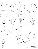
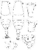
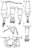
Acartia sp. Bradford, 1976 (p.181, figs.F,M). | | | | Ref.: | | | Bradford, 1976 (p.176, figs.F,M, Rem.); Ueda, 1986 (p.124, Redescr., figs.F,M, Rem.); 1986 b (p.134, figs.F,M); Kang & Lee, 1990 (p.378, figs.F,M, Rem.); Yoo & al., 1991 (p.258); Durbin E.G. & al., 1992 (p.342, Rem.: p.343, affinities with A. clausii); Samatov & Samatova, 1996 (p.21, figs.F, M, Rem.); Chihara & Murano, 1997 (p.670, Pl.16: F,M); Bradford-Grieve, 1999 (N°181, p.4, figs.F,M); Barthélémy, 1999 (p.858, 862, figs.F); 1999 a (p.9, Fig.22, C, D); Soh & Suh, 2000 (p.332); Caudill & Bucklin, 2004 (p.91, molecular biology); G. Harding, 2004 (p.22, figs.F,M); Zhang H. & al., 2013 (p.57, RNA-extraction method); Blanco-Bercial & al., 2014 (p.5, 6 , Rem.: problematic taxa) | 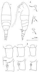 issued from : J.M. Bradford in N.Z. J. Mar. Freshw. Res., 1976, 10 (1). [p.176, 177, Figs.14,15]. Female (from East USA: Patuxent River, Gulf of Maine): 1a, habitus (dorsal view); 1b, idem (lateral view); 1c-e, P5.; 2a-c, genital segment (dorsal view); 2d-f, idem (lateral view).
|
 issued from : J.M. Bradford in N.Z. J. Mar. Freshw. Res., 1976, 10 (1). [p.178, Fig.16]. Male (from East USA): a, habitus (dorsal view); b, idem (lateral view); c, posterior surface of P5; d, terminal segment of left P5.
|
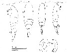
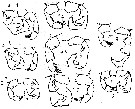
 issued from : H. Ueda in J. Oceanogr. Soc. Japan, 1986, 42 (2). [p.125, Fig.1]. Female (from different regions): A, B, urosome (dorsal and lateral, respectively; from Long Island Sound); C, D, urosome (lateral; from Chesapeake Bay); E, F, urosome (dorsal and lateral, respectively; from Maizuru Bay, Japan); G, H, idem (from San Juan Island, Puget Sound, Washington). Male: I, P5 (anterior view; Long Island Sound); J, idem (Maizuru Bay); K, idem (from San Juan Island).
|
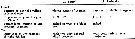
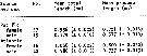
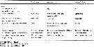
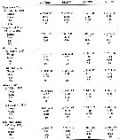 issued from : H. Ueda in J. Oceanogr. Soc. Japan, 1986, 42 (2). [p.125, Fig.1]. Female (from different regions):Prosome length and body proportions of Acartia hudsonica females from various Atlantic and Pacific localities. PL and PW: prosome length and width; GL and GW: genital segment length and width; RL and RW: right caudal ramus length and width.
|
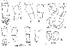
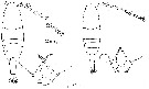
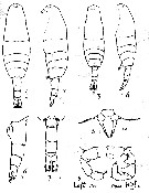
 issued from : H. Ueda in J. Oceanogr. Soc. Japan, 1986, 42. [p.136, Fig.2]. Comparative aspects between A. omorii, A. hudsonica and A. clausi. A. omorii (from Maizuru Bay, Japan): Female: A-B, urosome (dorsal and lateral, respectively);. Male: C, P5 (posterior view); D-E, 3rd segment of right P5 (other specimens). A. hudsonica (from Maizuru): Female: F-G, urosome (dorsal and lateral); H, P5 (posterior view); I-J, 3rd segment of right P5 (other specimens). A. clausi (after Bradford, 1976): Female: K-L, genital segment (dorsal and lateral, respectively).
|
 issued from : H. Ueda in J. Oceanogr. Soc. Japan, 1986, 42. [p.136, Table 1]. Comparative list of distinctive characters of A. omorii and A. hudsonica, after Bradford, 1976.
|
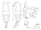
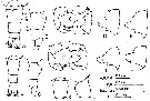
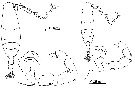
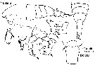
 issued from : J.M. Bradford in N.Z. J. Mar. Freshw. Res., 1976, 10 (1). [p.180, Fig.17]. As Acartia sp. Female (from San Juan Island, Puget Sound): a-b, habitus (lateral and dorsal, respectively); c, P5. Male: d-e, habitus (dorsal and lateral, respectively); f, P5 (anterior surface); g, basipod 2 of left P5 (posterior surface); h, terminal segment of left P5.
|
 issued from : J.M. Bradford in N.Z. J. Mar. Freshw. Res., 1976, 10 (1). [p.182, Fig.18]. As Acartia sp. Female (from Bremerton, Puget Sound): a-b, habitus (dorsal and lateral, respectively); c, P5. Male: d-e, habitus (dorsal and lateral, respectively); f, habitus of small form (dorsal); g, P5 (anterior surface); h, terminal segment of left P5.
|
 issued from : J.M. Bradford in N.Z. J. Mar. Freshw. Res., 1976, 10 (1). [p.183, Fig.19]. As Acartia sp. Female (from Puget Sound): a-b, habitus (lateral and dorsal, respectively). Male: c-d, habitus (dorsal and lateral , respectively); e, P5 (anterior surface). Nota: having subsequently seen female from Puget Sound with or without small spinules posterodorsally on the urosome segments and males in which the proportions of the right caudal ramus straddle the two previous forms, the author looks at as one variable species.
|
 issued from : E.B.-G. Carillo, C.B. Miller and P.H. Wiebe in Limnol. Oceanogr., 1974, 19 (3). [p.455, Fig.2]. As Acartia clausi. Females (from Yaquina Bay, Oregon;) (right figure) and Acartia clausi (from Woods Hole: Atlantic form) (left figure). Interbreeding attempts between Atlantic and Pacific populations.
|
 issued from : E.B.-G. Carillo, C.B. Miller and P.H. Wiebe in Limnol. Oceanogr., 1974, 19 (3). [p.455, Fig.1]. As Acartia clausi. Male (from Yaquina Bay, Oregon) (right figure) and Acartia clausi (from Woods Hole) (left figure) (left figure). Interbreeding attempts between Atlantic and Pacific populations.
|
 issued from : E.B.-G. Carillo, C.B. Miller and P.H. Wiebe in Limnol. Oceanogr., 1974, 19 (3). [p.456, Table 3]. As Acartia clausi. Sizes of adult Acartia clausi from Pacific and Atlantic forms cultured at 17°C. Interbreeding attempts between Atlantic and Pacific populations. Atlantic males and females are bigger than pacific males and females; the shape of the 4th segment of the male urosome is different: in the Atlantic form it bears a triangular projection pointing posteriorly on the dorsal side, in the Pacific male the projection is indented at the midline; P5 of females are very similar; P5 males of the Atlantic form are relatively bigger than those of the Pacific form. The Atlantic and Pacific populations of Acartia clausi (largo sensu) have been grouped for mabny years under the same name, based on morpholological similarity (Esterly, 1924). The comparisons between individuals shows differences mostly by size, and by a few subtle details in the males. mayr (1963) pointed out that most geographic isolates differ in some morphologic characters. These differences are not necessarily evidence of reproductive isolation, but are frequently correlated with it. The authors have shown experimentally that under the same environmental conditions, Atlantic and Pacific populations were able separately to breed and produce fertile off-spring, but not when members of the two populations were brought together. It is not yet clear that either the Pacific or Atlantic population with interbreeding potentiallity possible between all of its geographic wide area; the assignment of new specific names should only follow a larger, possibly worldwide study of Acartia clausi populations. The authors follow in this the taxonomic philosophy of Wilson & Brown (1953). Physiomogical, ecological, and behavorial differences have been found in closely related and similar species. According to Mayr (1963), this indicates that each is a separate biological system with species specific tolerances to physical and biological factors.
|
 issued from : Y.-S. Kang & S.-S. Lee in Bull. Korean Fish. Soc., 1990, 23 (5). [p.381, Fig.2]. Female (from Korea): D, habitus (dorsal); E, 1st, 2nd urosomal segments (dorsal); F, genital segment (lateral). Male: A, habitus (dorsal); B, P5; C, inner lobe of 3rd segment of right P5.
|
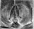 issued from : R.-M. Bathélémy in J. Mar. Biol. Ass. U.K., 1999, 79. [p.860, Fig.3, C]. Scanning electon miccrograph. Female (from Maizuru Bay, Japan): C, genital area (external ventral view). Scale bar: 0.030 mm. Symbols: * = fixation site of the spermatophore; arrowhead = lamellar flap.
|
 issued from : L. Seuront in J. Plankton Res., 2005, 27 (12). [p.1303, Table I]. Comparisons of distinctive characters of Acartia closely related to each other.
|
 issued from : G. Harding in Key to the adullt pelagic calanoid copepods found over the continental shelf of the Canadian Atlantic coast. Bedford Inst. Oceanogr., Dartmouth, Nova Scotia, 2004. [p.22]. Female & Male
|
 Issued from : M. Chihara & M. Murano in An Illustrated Guide to Marine Plankton in Japan, 1997. [p.674, Pl. 16, fig.4 a-g]. Female: a, habitus (dorsal); b, last thoracic segment and urosome (dorsal); c, same (lateral, right side); d, P5. Male: e, habitus (dorsal); f, last thoracic segment and urosome (dorsal); g, P5 d, P5. Nota: numbers show caracteristics of this species to compare with A. omorii.
|
 Issued from : H.Y. Soh & H.-L. Suh in J. Plankton Res., 2000, 22 (2). [p.332, Table I]. Distinctive characters of Acartia hudsonica. Nota: Compare the distinctive characters with the closely related species A. omorii, A. hongi in the coastal waters of Korea, and A. bifilosa.
|
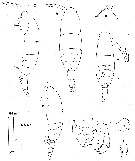
 Issued from : A.D. Samatov & I.N. Samatova in Biol. Mor., 1996, 22 (1). [p.23, Fig.2]. Female (from 53°N, 158°30' E): 1-2, habitus (dorsal and lateral , respectively); 5, P5; 6, abdomen (lateral view). Male: 3-4, habitus (dorsal and lateral, respectively); 7, abdomen (lateral view); 8, P5 (lL: left leg; R: right leg). Nota: The females can be idebtified by long genital segment with genital swelling located entirely in the anterior half of the former. The males distinguish by naked urosomal segments and by undivided rounded lobe of the 3rd segment of right P5.
|
 Issued from : A.D. Samatov & I.N. Samatova in Biol. Mor., 1996, 22 (1). [p.24, Fig.3]. Morphology of the P5 male in Acartia hudsonica: 1 - after Bradford, 1976 (p.180, fig.17f); 2 - after Ueda, 1986a (p.125, fig.1I); 3 - after Ueda, 1986b (p.136, fig.1H); 4 - after Brodsky, 1950 (c.420, fig.296); 5 - after Bradford, 1976 (p.178, fig.16c. Acartia sp.); 6 -,after Bradford, 1976 (p.182, fig?18g). Acartia omorii: 7 - after Bradford, 1976 (p.175, fig.13c); 8 - after Ueda, 1986 b (p.136, fig.2C).
| | | | | Ref. compl.: | | | Conover, 1978 (p.66, 72, feeding); Deason, 1980 (p.101, grazing); Hebert & Poulet, 1980-81 (p.121, feeding vs. oil polluant); Turner & Dagg, 1983 (p.16); Turner & Anderson, 1983 (p.359, grazing); McLaren & Marcogliese, 1983 (p.721, cell nucleus); Tremblay & Anderson, 1984 (p.3, Rem.); Hargrave & al., 1985 (p.221, annual abundance); Sullivan & McManus, 1986 (p.121, resting egg production); Ueda, 1987 (p.691); Bollens & Frost, 1989 (p.1047, vertical migration vs predator); Verity & Smayda, 1989 (p.161, ingestion-egg production); Stoecker & McDowell Capuzzo, 1990 (p.891, feeding); Gifford, 1991 (p.8, Table 2, diet); Huntley & Lopez, 1992 (p.201, Table 1, eggs, temperature-dependent production); Durbin & al., 1992 (p.342, size-weight, egg production); Durbin A.G. & Durbin, 1992 (p.379, egg development, age distribution); Durbin E.G. & Durbin, 1992 a (p.361, feeding, length-weight, temperature effect); Rodriguez & Durbin, 1992 (p.7, feeding behaviour); Yen & Fields, 1992 (p.123, nauplli vs. predator); Kimmerer, 1993 (tab.2); Weissman & al., 1993 (p.613, epibiontic effects); Jonasdottir, 1994 (p.67, nutrition vs reproduction); Bollens & al., 1994 (p.555, vertical migration/predators); Landry & al., 1994 (p.55, abundance, grazing); Marcus & al., 1994 (p.154, Rem. p.157); Ohtsuka & al., 1995 (p.158: Rem., 159); Samatov & Samatova, 1996 (p.21); Madhupratap & al., 1996 (p.77, Table 2: resting eggs); Marcus, 1996 (p.143); Mauchline, 1998 (p.525, tab.19, 21, 33, 40, 45, 63, 64); Gomez-Gutiérrez & Peterson, 1999 (p.637, Table II, abundance); Ueda & al., 2000 (tab.1); White & McLaren, 2000 (p.751, tab.1); Uye & al., 2000 (p.193, fig.8 : abundance vs t°, Sal.); Peterson & al., 2002 (p.353); Peterson & al. 2002 (p.381, Table 2, interannual abundance); Mackas & Galbraith, 2002 (p.725, tab.2a, 2b); Peterson & Keister, 2003 (p.2499, interannual variability); Keister & Peterson, 2003 (p.341, Table 1, 2, abundance, cluster species vs hydrological events); Shimode & Shirayama, 2004 (tab.2); Mackas & al., 2004 (p.875, Table 2); Choi & al., 2005 (p.710: Tab.III); Manning & Bucklin, 2005 (p.233, Table 1, fig.12); Mackas & Coyle, 2005 (p.707, fig.7); Miller C.B., 2005 (p.152: life history, figs.7.15, 7.16, production: fig.7.17, table 7.1); Mackas & al., 2006 (L22S07, Table 2); Hooff & Peterson, 2006 (p.2610); Sullivan & al., 2007 (p.259, Rem.: climate change); Colin & Dam, 2007 (p.875, toxic effect); Sullivan & al., 2008 (p.485); Makino & al., 2008 (p.639: feeding rates); Teegarden & al., 2008 (p.33, Rem.: feeding and toxicity); Humphrey, 2008 (p.83: Appendix A); Yen & al., 2008 (p.283, Rem.: kinematic); Ohtsuka & al., 2008 (p.115, Table 4, 5); Peterson, 2009 (p.73, Rem.: p 78); Hopcroft & al., 2009 (p.9, Table 3); Hopcroft & al., 2010 (p.27, Table 2, fig.9); Yen & Lasley, 2010 (p.177, fig. 9.6, Rem.: p.183, 189, mating); Milligan & al., 2011 (p.155, phylogeography); Zheng Y. & al., 2011 (p.723, toxic food); Dam & Haley, 2011 (p.245, dinoflagellate toxicity effect); Sakaguchi & al., 2011 (p.18, Table 1, occurrences); Senft & al., 2011 (p.804, ingestion rate vs dinoflagellate toxins); Turner & al., 2011 (p.1066, Table II, abundance 1998-2008); Kang J.-H., 2011 (p.219, occurrences, inter-annual variability vs t° & Sal., Chl.a, Rem.: p.224); Matsuno & al., 2011 (p.1349, Table 1, abundance vs years); Haley & al., 2011 (p.927, grazing vs PCR identification); Beltrao & al., 2011 (p.47, Table 1, density vs time); DiBacco & al., 2012 (p.483, Table S1, ballast water transport); Moon & al., 2012 (p.1, Table 1, 2, figs.10, 11, seasonal & spatial variations); Takahashi M. & al., 2012 (p.393, Table 2, water type index); Seo & al., 2013 (p.448, Table 1, occurrence), Gusmao & al., 2013 (p.279, Table 3, sex-specific predation by fish); Questel & al., 2013 (p.23, Table 3, interannual abundance & biomass, 2008-2010); Eisner & al., 2013 (p.87, Table 3: abundance vs water structure); Rice & al., 2014 (p.23, fig.3, size vs. years 1952-2011, climate change); Ohtsuka & Nishida, 2017 (p.565, 578, Table 22.1, Fig.22.3: central station-innermost station in Japanese waters); Baumgartner & Tarrant, 2017 (p.387, resting eggs, fig.5, Rem.). | | | | NZ: | 7 | | |
|
Carte de distribution de Acartia (Acartiura) hudsonica par zones géographiques
|
| | | | | |  Carte de 1996 Carte de 1996 | |
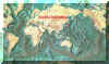
 issued from : H. Ueda in J. Oceanogr. Soc. Japan, 1986, 42. [p.136, Fig.1]. issued from : H. Ueda in J. Oceanogr. Soc. Japan, 1986, 42. [p.136, Fig.1].
Distribution of A. omorii and A. hudsonica in Japanese inlet and cosatal waters. |
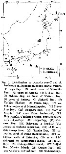
 issued from : Y.-S. Kang & S.-S. Lee in Bull. Korean Fish. Soc., 1990, 23 (5). [p.383, Fig.4]. issued from : Y.-S. Kang & S.-S. Lee in Bull. Korean Fish. Soc., 1990, 23 (5). [p.383, Fig.4].
Distribution of Acartia hudsonica and Acartia omorii in Korean waters: 1: Sogcho; 2: ChumunJin; 3: UlJin; 4: Pusan; 6: ChejuDo; 7: Taeheugsan-Do; 8: Young-kwang. |
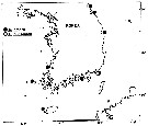
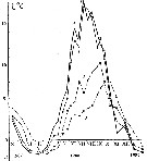
 issued from : B.T. Hargrave, G.C. Harding, K.F. Drinkwater, T.C. Lambert & W.G. Harrison in Mar. Ecol. Prog. Ser., 1985, 20. [p.227, Fig.7]. issued from : B.T. Hargrave, G.C. Harding, K.F. Drinkwater, T.C. Lambert & W.G. Harrison in Mar. Ecol. Prog. Ser., 1985, 20. [p.227, Fig.7].
Major species of zooplankton present at the central station in St. Georges Bay (45°45'N, 61°45'W) during 1977.
Nota: All zooplankton collections were made after sunset. The net towed obliquely throughout the water column (± 34 m in depth). |
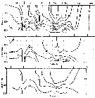 issued from : B.T. Hargrave, G.C. Harding, K.F. Drinkwater, T.C. Lambert & W.G. Harrison in Mar. Ecol. Prog. Ser., 1985, 20. [p.223, Fig.2]. issued from : B.T. Hargrave, G.C. Harding, K.F. Drinkwater, T.C. Lambert & W.G. Harrison in Mar. Ecol. Prog. Ser., 1985, 20. [p.223, Fig.2].
Seasonal profiles of water temperature and salinity in St. Georges Bay (45°45'N, 61°45'W) near the central station during 1977. |
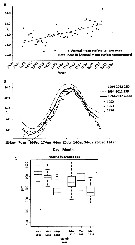 Issued from : E. Rice, H.G. Dam & G. Stewart in Estuaries and Coasts, 2014. [p.17, Fig.2, A, B; Fig.3, C]. Issued from : E. Rice, H.G. Dam & G. Stewart in Estuaries and Coasts, 2014. [p.17, Fig.2, A, B; Fig.3, C].
A: Inshore Central Basin of Long Island Sound trend of temperature over 1978-2012. Correlation coefficient (tau) = 0.49, p <<0.01. Line shownh is the best fit, slope = 0.03, intercept = -43.2. N = 63. Data from the NOAA Milford Laboratory.
B: Off shore surface temperatures for Central Basin stations (mean and 2SD) for 1994-2012 and reported values from Riley & al. (1986) for 1952-1954.
C: Box-and-whisker plot of mean prosome lengths (µm) of Acartia hudsonica during March and May 1952, 2010, and 2011. The thick, center line in each box is the median; upper and lower solid lines of the box represent the first and third quartiles, respectively; dashed lines represent the range; and open circles are outlies. |
 Issued from : A.D. Samatov & I.N. Samatova in Biol. Mor., 1996, 22 (1). [p.25, Fig.4]. Issued from : A.D. Samatov & I.N. Samatova in Biol. Mor., 1996, 22 (1). [p.25, Fig.4].
Seasonal dynamics of the copepod Acartia hudsonica in the Avachinskaya Bay (Southeastern Kamchatka) during November 1987 to February 1989 .
1: nauplii; 2: copepodites; 3: adultes. a: number; b: mg/m3.
Samatov abd Samatova (1996) note that the abundant copepod formerly identified in coastal waters of the Northern Pacific as Acartia clausi was redefined after examination of specimens from Avachinskay Bay (SE Kamchatka). This species is well distinguished from closely related Pacific species A. omorii and Acartia sp. from Puget Sound. Probably three generations by year. |
 Issued from : A.D. Samatov & I.N. Samatova in Biol. Mor., 1996, 22 (1). [p.25, Fig.5]. Issued from : A.D. Samatov & I.N. Samatova in Biol. Mor., 1996, 22 (1). [p.25, Fig.5].
Annual variation of the salinity (p.1000) in the Avachinskaya Bay (SE Kamcharka).
1- surface mean; 2- 10 m depth; 3- in the bottom; 4- in surface at the station 2. (western Bay). |
 Issued from : A.D. Samatov & I.N. Samatova in Biol. Mor., 1996, 22 (1). [p.25, Fig.6]. Issued from : A.D. Samatov & I.N. Samatova in Biol. Mor., 1996, 22 (1). [p.25, Fig.6].
Annual variation of the temperature (°C).
1- surface mean; 2- 10 m depth; 3- in the bottom; 4- in surface at the station 2. (western Bay). |
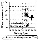 Issued from : J.-H. Kang in Ocean Sci. J., 2011, 46 (4). [p.228, Fig.5] Issued from : J.-H. Kang in Ocean Sci. J., 2011, 46 (4). [p.228, Fig.5]
Abundance-temperature-salinity diagram of A. hudsonica observed in the seaports from Korea during 3 years (2007-2009). |
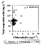 Issued from : J.-H. Kang in Ocean Sci. J., 2011, 46 (4). [p.229, Fig.6] Issued from : J.-H. Kang in Ocean Sci. J., 2011, 46 (4). [p.229, Fig.6]
Abundance-total suspended solid-chlorophyll-a diagram of A. hudsonica observed in the seaports from Korea during 3 years (2007-2009). |
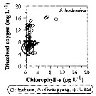 Issued from : J.-H. Kang in Ocean Sci. J., 2011, 46 (4). [p.230, Fig.7] Issued from : J.-H. Kang in Ocean Sci. J., 2011, 46 (4). [p.230, Fig.7]
Abundance-dissolved oxygen-chlorophyll-a diagram of A. hudsonica observed in the seaports from Korea during 3 years (2007-2009). |
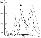
 Issued from : C.B. Miller in Biological Oceanography 2004/2005, Blackwell Publishing. [p.139, Fig.7.5]. Issued from : C.B. Miller in Biological Oceanography 2004/2005, Blackwell Publishing. [p.139, Fig.7.5].
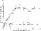
Shift in the asymptote of the ingestion rate curve in Acartia hudsonica from Yaquina Bay, Oregon between May and June (lower curves) and July and August (upper curves). When food is more abundabt in the field (summer in this estuary), more food is consumed than when it is sparser (spring). (Afeter Donaghay P.L., 1980, PhD Dissertation, Oregon State University). |
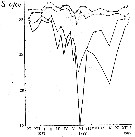
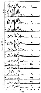 Issued from : C.B. Miller in Biological Oceanography 2004/2005, Blackwell Publishing. [p.153, Fig.7.15]. After Landry, 1978. Issued from : C.B. Miller in Biological Oceanography 2004/2005, Blackwell Publishing. [p.153, Fig.7.15]. After Landry, 1978.
Stacked time of stage estimates for Acartia hudsonica in Jakle's Lagoon (Washington State, USA) in 1973. Groups (I throughj VI) identified as ''cohorts'' are alternately shaded or white [suppose six generations during the year]. |
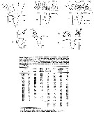
 Issued from : C.B. Miller in Biological Oceanography 2004/2005, Blackwell Publishing. [p.157, Table 7.1]. After Landry, 1978. Issued from : C.B. Miller in Biological Oceanography 2004/2005, Blackwell Publishing. [p.157, Table 7.1]. After Landry, 1978.
Calanus pacificus dominant zooplankters in the Jakle's Lagoon (near Puget Sound). Data characterize the season of peak production: 70-55 mgC m-2 day-1 (estimates for 2 years).
Miller underlines the difficulties of the production estimations for single species, and virtually none for whole systems, but we would like to know how much food the oceans produces for animals we harvest like herring, anchovy, cod, and pollack. See Huntley & Lopez, 1992: model); Kleppel, Davis & Carter, 1996; Huntley, 1996; Hirst & Sheader, 1997; Hirst & Lampitt, 1998; Vidal, 1980. |
 Issued from J. Yen & D.M. Fields in Arch. Hydribiol. Beih. Ergebn. Limnol., 1992, 36 [p.127: Fig.2; p.128: Fig.3; p.130: Figs.4, 5, 6; p.131: Table 1]. Escape responses of A. hudsonica nauplii from the flow field of Temora longicornis. Issued from J. Yen & D.M. Fields in Arch. Hydribiol. Beih. Ergebn. Limnol., 1992, 36 [p.127: Fig.2; p.128: Fig.3; p.130: Figs.4, 5, 6; p.131: Table 1]. Escape responses of A. hudsonica nauplii from the flow field of Temora longicornis.
A: Illustration of the flow field (3.5 mm across by 1.9 mm) representing the velocity gradient within 560 µm corridor above the first antennae of T. longicornis. Each arrow represents 1/6 sec of travel. The eight streamlines were mapped from a total of 98 data points.
B: Contour map of equal velocity constructed from the flow field within the corridor above the first antennae of T. longicornis.
C:. Velocities reached 2 mm/s at a distance of 0.5 mm above the tip of the prosome Positions within the corridor above the first antennae of T. longicornis of the points of escape exhibited by the nauplii (250 µm) of A. hudsonica relative to the velocity contours (mm/s). Solid circles represent the first escape (n = 20) while open circles represent subsequent escapes (n = 29)
Note how close some of the nauplii got to the central region of the flow field above the first antennae, while in the region where the velocity contours are curved, excapes are executed farther away from the copepod.
D: Trajectory of a nauplius of A. hudsonica that became entrained within the flow field of T. longicornis and tried to escape several times.
The view from one camera gave the x, z positions and the view from the other camera gave y, z positions. Cameras were oriented at right angles to each other. Each dot followed the movement of the nauplii 1/6 s apart while arrows depicting jumps were 1/30 apart. Tiny dots illustrated a jump back to original position.
E: Illustration of the model used to compute shear of the nauplii at their points of escape over a span (250 µm) of their sensors on a plane perpendicular (solid line) to the streamlines. Dotted lines were drawn parallel through the streamlines.
Three dimensional visualization of escapes of nauplii (250 µm) from the flow field created by a predator (Temora longicornis) permitted analyses of hydrodynamic cues at temporal and spatial scales. Within a narrow corridor above the the predator's primary sensors (the A1), the points of escape by the nauplii were mapped.
The velocity of the nauplius at the point of escape was compared to the velocity gradient of the flow field. It is found large variability in: a- the average acceleration of 0.53 mm/s2 ± 120.5, computed along the streamline over a time interval corresponding to a distance travelled of one body length; b- the average shear of 0.80/s ± 84.5 %, computed perpendicular to the streamline over a distance equivalent to the span of the sensor; c- the average relative velocity, where the velocity of the nauplius was 0.74 ± 27.1% that of the surrounding water.
To avoid predation, nauplli should rely on a cue that minimizes the risk of capture. Since most distant escapes occurred where velocity contours were curved (high shear), shear was considered the cue to alert nauplii to the presence of the predator.
Distance to the predator and velocity of the nauplius were not considered potential cue because: 1- distance cannot be perceived nonvisually: 2- within a temporally-constant and spatially-uniform velocity ,gradient, the movement of the nauplii follows that of the water; constant velocity causes no setal bending which is necessary for the perception of water movement. When the fluid is moving faster than the nauplius body, the setae, which follow the fluid movement, are bent relative to the body which lags in the fluid.
Strategically, the escape response of the prey to the hydrodynamic cue should minimize the risk of capture. In figure C, many of the distant escapes occurred in areas where the velocity contours are curved which corresponds to areas of high shear while some escapes occurred in the central region close to the mouth where acceleration is high. |
| | | | Loc: | | | NW Atlant. (Strait of Belle Isle, Perch Pond (Falmouth, Massachusetts), Tuckerton Bay, Hudson Bay, Patuxent River, Long Island Sound, Rhode Island (Pettaquamscutt estuary, Narragansett Bay), G. of Maine, Chesapeake Bay, Bay of Fundy, Nova Scotia, Bedford Basin, James Bay, Passamoquoddy Bay, Casco Bay, Halifax Harbor, St. Lawrence Estuary (Rimouski), St. Georges Bay, Long Island, Cape Cod, Great Bay, Norfolk (Virginia), ? China Seas, Korea, Incheon Harbour, Muan Bay, Japan (Akkeshi Bay, Ariake Bay,, Tanabe Bay, Maizuru Bay, Shiogama Bay, Honshu: Okkirai Bay, Lake Nakaumi), California, Santa Monica Basin, Jakle's Lagoon (marine pond adjacent to Puget Sound), Oregon (coast, off Newport), San Francisco Bay, Tomales Bay, San Juan Is., British Columbia, Queen Charlotte Is., ? S Beaufort Sea, ? Alaska (Port Clarence), SE Kamchatka (Avachinskaya Bay), Chukchi Sea | | | | N: | 96 | | | | Lg.: | | | (174) F: 1,07-0,87; M: 0,96-0,81; (181)* F: 1,32-0,74; M: 1,07-0,71; (866) F: 0,8-1,2; M: 0,7-1; (1089) F: 0,87-1,2; M: 0,81-1,02; (1221) F: 1,06-1,27 (May); M:0,91-1,12 (April); M: 0,62-1,08 (May); 0,82-0,94 (April); (1309) F: 0,85-1,308; {F: 0,74-1,32; M: 0,71-1,07}
*: F: 1,0-1,32 (Chesapeake Bay, March); F: 1,05-1,13; M: 0,97-1,07 (Long Island Sound, June); F: 0,92-1,10 (March); M: 0,86-0,93 (March); F: 0,81-0,92 (June) (Maizuru Bay); F: 1,09-1,17 (May); M: 0,94-1,0 (May); F: 0,78-0,95 (August) (Akkeshi Bay); F: 0,74-0,85; M: 0,71-0,84 (San Juan Island, May). | | | | Rem.: | Certaines confusions avec Acartia clausi rendent certaines localisations incertaines dans le Pacifique comme en Atlantique.
Voir aussi les remarques en anglais | | | Dernière mise à jour : 22/10/2020 | |
|
|
 Toute utilisation de ce site pour une publication sera mentionnée avec la référence suivante : Toute utilisation de ce site pour une publication sera mentionnée avec la référence suivante :
Razouls C., Desreumaux N., Kouwenberg J. et de Bovée F., 2005-2025. - Biodiversité des Copépodes planctoniques marins (morphologie, répartition géographique et données biologiques). Sorbonne Université, CNRS. Disponible sur http://copepodes.obs-banyuls.fr [Accédé le 27 août 2025] © copyright 2005-2025 Sorbonne Université, CNRS
|
|
|
|


 hudsonica - Planche 1 de figures morphologiques',750,500);)
 hudsonica - Planche 2 de figures morphologiques',750,500);)
 hudsonica - Planche 3 de figures morphologiques',750,500);)
 hudsonica - Planche 4 de figures morphologiques',750,500);)
 hudsonica - Planche 5 de figures morphologiques',750,500);)
 hudsonica - Planche 7 de figures morphologiques',750,500);)
 hudsonica - Planche 8 de figures morphologiques',750,500);)
 hudsonica - Planche 9 de figures morphologiques',750,500);)
 hudsonica - Planche 10 de figures morphologiques',750,500);)
 hudsonica - Planche 11 de figures morphologiques',750,500);)
 hudsonica - Planche 13 de figures morphologiques',750,500);)
 hudsonica - Planche 14 de figures morphologiques',750,500);)
 hudsonica - Planche 15 de figures morphologiques',750,500);)
 hudsonica - Planche 16 de figures morphologiques',750,500);)
 hudsonica - Planche 17 de figures morphologiques',750,500);)
 hudsonica - Planche 18 de figures morphologiques',750,500);)
 hudsonica - Planche 19 de figures morphologiques',750,500);)
 hudsonica - Planche 20 de figures morphologiques',750,500);)

 hudsonica - Carte de distribution 2',650,500);)
 hudsonica - Carte de distribution 3',750,500);)
 hudsonica - Carte de distribution 4',750,500);)
 hudsonica - Carte de distribution 5',750,500);)
 hudsonica - Carte de distribution 6',750,500);)
 hudsonica - Carte de distribution 7',750,500);)
 hudsonica - Carte de distribution 8',750,500);)
 hudsonica - Carte de distribution 9',750,500);)
 hudsonica - Carte de distribution 10',750,500);)
 hudsonica - Carte de distribution 11',750,500);)
 hudsonica - Carte de distribution 12',750,500);)
 hudsonica - Carte de distribution 13',750,500);)
 hudsonica - Carte de distribution 14',750,500);)
 hudsonica - Carte de distribution 15',750,500);)
 hudsonica - Carte de distribution 17',750,500);)
 hudsonica - Planche 1 de figures morphologiques)
 hudsonica - Planche 2 de figures morphologiques)
 hudsonica - Planche 3 de figures morphologiques)
 hudsonica - Planche 4 de figures morphologiques)
 hudsonica - Planche 5 de figures morphologiques)
 hudsonica - Planche 6 de figures morphologiques)
 hudsonica - Planche 7 de figures morphologiques)
 hudsonica - Planche 8 de figures morphologiques)
 hudsonica - Planche 9 de figures morphologiques)
 hudsonica - Planche 10 de figures morphologiques)
 hudsonica - Planche 11 de figures morphologiques)
 hudsonica - Planche 12 de figures morphologiques)
 hudsonica - Planche 13 de figures morphologiques)
 hudsonica - Planche 14 de figures morphologiques)
 hudsonica - Planche 15 de figures morphologiques)
 hudsonica - Planche 16 de figures morphologiques)
 hudsonica - Planche 17 de figures morphologiques)
 hudsonica - Planche 18 de figures morphologiques)
 hudsonica - Planche 19 de figures morphologiques)
 hudsonica - Planche 20 de figures morphologiques)
 hudsonica - Carte de distribution 2)
 hudsonica - Carte de distribution 3)
 hudsonica - Carte de distribution 4)
 hudsonica - Carte de distribution 5)
 hudsonica - Carte de distribution 6)
 hudsonica - Carte de distribution 7)
 hudsonica - Carte de distribution 8)
 hudsonica - Carte de distribution 9)
 hudsonica - Carte de distribution 10)
 hudsonica - Carte de distribution 11)
 hudsonica - Carte de distribution 12)
 hudsonica - Carte de distribution 13)
 hudsonica - Carte de distribution 14)
 hudsonica - Carte de distribution 15)
 hudsonica - Carte de distribution 16)
 hudsonica - Carte de distribution 17)