|
|
 |
Fiche d'espèce de Copépode |
|
|
Calanoida ( Ordre ) |
|
|
|
Calanoidea ( Superfamille ) |
|
|
|
Paracalanidae ( Famille ) |
|
|
|
Calocalanus ( Genre ) |
|
|
| |
Calocalanus pavo (Dana, 1849) (F,M) | |
| | | | | | | Syn.: | Ctenocalanus pavo : lapsus calami in Seridji & Hafferssas, 2000 (tab.1);
? Calocalanus parvus : Hopcroft & al., 1998 (tab.2, lapsus calami)
Calocalanus pavus : Tutasi & al., 2011 (p.791, Table 2, abundance distribution vs La Niña event); | | | | Ref.: | | | Giesbrecht, 1892 (p.175, 185, 770, figs.F,M); T. Scott, 1894 b (p.37, figs.F); Giesbrecht & Schmeil, 1898 (p.26, Rem. F,M); Wheeler, 1901 (p.169, fig.F, Rem.); Thompson & Scott, 1903 (p.233, 243); A. Scott, 1909 (p.30, Rem.); Wolfenden, 1911 (p.203); Sewell, 1912 (p.353, 359); 1914 a (p.213); Pesta, 1920 (p.501); Früchtl, 1924 b (p.42); Farran, 1929 (p.208, 222); Sewell, 1929 (p.89); Wilson, 1932 a (p.39, fig.F); Rose, 1933 a (p.78, figs.F,M); Farran, 1936 a (p.83); Mori, 1937 (1964) (p.33, figs.F); Vervoort, 1946 (p.138, Rem.); Sewell, 1947 (p.54); Farran & Vervoort, 1951 d (n°36, p.3, figs.F,M); Marques, 1953 (p.96); Chiba, 1956 (p.30, figs.F juv.); Tanaka, 1956 c (p.377); Chiba & al., 1957 (p.306); 1957 a (p.11); Tanaka, 1960 (p.29); Bernard, 1960 (n°36 first revision, p.3, figs.F,M); Fish, 1962 (p.13); Grice, 1962 (p.187, fig.F); Brodsky, 1962 c (p.115, figs.F); Vervoort, 1963 b (p.113, Rem.); Paiva, 1963 (p.26); Kasturirangan, 1963 (p.20, figs.F,M); Tanaka, 1964 (p.6); Chen & Zhang, 1965 (p.43, figs.F); Saraswathy, 1966 (1967) (p.76); Owre & Foyo, 1967 (p.39, figs.F,M, Rem.); Park, 1968 (p.540); Vidal, 1968 (p.23, figs.F); Vilela, 1968 (p.12); Corral Estrada, 1970 (p.112, figs.F,M, Rem.); Razouls, 1972 (p.94, Annexe: p.22, fig.F); Corral, 1972 b (n°138, p.4, figs.F,M); Björnberg, 1972 (p.19, figs., Rem.N); Chen & Zhang, 1974 (p.107, figs.M); Marques, 1974 (p.13, fig.F); 1976 (p.989); Dawson & Knatz, 1980 (p.4, figs.F,M); Björnberg & al., 1981 (p.626, figs.F,M); Schnack, 1982 (p.145, fig.Md); Zheng & al., 1982 (p.24, figs.F). Sazhina, 1985 (p.42, figs.N); Zheng Zhong & al., 1989 (p.233, figs.F); Schnack, 1989 (p.137, tab.1, fig.6: Md); Bradford-Grieve, 1994 (p.59, figs.F,M, fig.99); Chihara & Murano, 1997 (p.749, Pl.71: F,M); Bradford-Grieve & al., 1999 (p.877, 909, figs.F,M); Conway & al., 2003 (p.157, figs.F,M, Rem.); Boxshall & Halsey, 2004 (p.154, figs.F,M); Mulyadi, 2004 (p.180, figs.F, Rem.); Avancini & al., 2006 (p.70, Pl. 39, figs.F,M, Rem.); Vives & Shmeleva, 2007 (p.951, figs.F,M, Rem.); Phukham, 2008 (p.121, figs.F); Andronov, 2014 (p.73, fig. P5 M) | 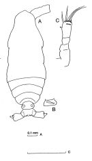 issued from : J.M. Bradford-Grieve in The Marine Fauna of New Zealand: Pelagic Calanoid Copepoda. National Institute of Water and Atmospheric Research (NIWA). New Zealand Oceanographic Institute Memoir, 102, 1994. [p.60, Fig.31]. Female: A, habitus (dorsal); B, lateral view of genital segment; C, P5.
|
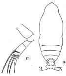 issued from: Q.-c Chen & S.-z. Zhang in Studia Marina Sinica, 1965, 7. [Pl.9, 16-17]. Female (from E China Sea): 16, habitus (dorsal); 17, right P5 (posterior).
|
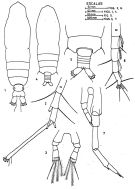 issued from : J. Corral Estrada in Tesis Doct., Univ. Madrid, A-129, Sec. Biologicas, 1970. [Lam.25]. Female (from Canarias Is.): 1, habitus (dorsal); 2, distal segments of A1; 3, P5. Male: 4, habitus (dorsal); 5, posterior part cephalothorax and urosome (dorsal); 6, distal segments of A1; 7, P5.
|
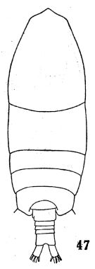 issued from : Q.-c. Chen & S.-z. Zhang in Studia Marina Sinica, 1974, 9. [Pl.4, Fig.47]. Male (from South China Sea): 47, habitus (dorsal).
|
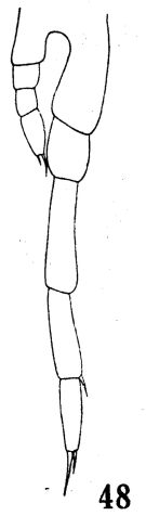 issued from : Q.-c. Chen & S.-z. Zhang in Studia Marina Sinica, 1974, 9. [Pl.5, Fig.48]. Male: 48, P5.
|
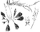 issued from : T. Mori inThe pelagic Copepoda from the neighbouring waters of Japan, 1937 (1964). [Pl.13, Figs.1-3]. Female: 1, habitus (dorsal); 2, P1 (posterior); 3, P5.
|
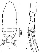 issued from : Z. Zheng, S. Li, S.J. Li & B. Chen in Marine planktonic copepods in Chinese waers. Shanghai Sc. Techn. Press, 1982 [p.24, Fig.11] Female: a, habitus (dorsal); b, P5. Scale in mm.
|
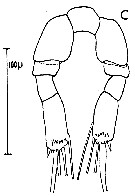 issued from : C. Razouls in Th. Doc. Etat Fac. Sc. Paris VI, 1972, Annexe. [Fig.27, C]. Female (from Banyuls, G. of Lion): C, P5.
|
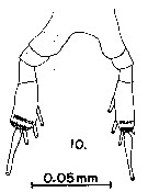 issued from : G.D. Grice in Fish. Bull. Fish and Wildl. Ser., 1962, 61. [p.186, Pl.6, Fig.10]. Female (from equatorial Pacific): 10, P5.
|
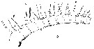 Issued from : W. Giesbrecht in Systematik und Faunistik der Pelagischen Copepoden des Golfes von Neapel und der angrenzenden Meeres-Abschnitte. – Fauna Flora Golf. Neapel, 1892, 19 , Atlas von 54 Tafeln. [Taf.9, Fig.3]. Female: 3, A1proximal segments; ventral view).
|
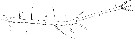 Issued from : W. Giesbrecht in Systematik und Faunistik der Pelagischen Copepoden des Golfes von Neapel und der angrenzenden Meeres-Abschnitte. – Fauna Flora Golf. Neapel, 1892, 19 , Atlas von 54 Tafeln. [Taf.9, Fig.4]. Female: 4, A1 (distal segments; ventral view).
|
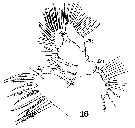 Issued from : W. Giesbrecht in Systematik und Faunistik der Pelagischen Copepoden des Golfes von Neapel und der angrenzenden Meeres-Abschnitte. – Fauna Flora Golf. Neapel, 1892, 19 , Atlas von 54 Tafeln. [Taf.9, Fig.16]. Female: 16, Mx1 (anterior view).
|
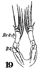 Issued from : W. Giesbrecht in Systematik und Faunistik der Pelagischen Copepoden des Golfes von Neapel und der angrenzenden Meeres-Abschnitte. – Fauna Flora Golf. Neapel, 1892, 19 , Atlas von 54 Tafeln. [Taf.9, Fig.19]. Female: 19, P5.
|
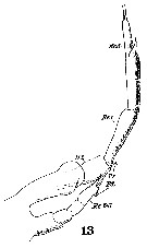 Issued from : W. Giesbrecht in Systematik und Faunistik der Pelagischen Copepoden des Golfes von Neapel und der angrenzenden Meeres-Abschnitte. – Fauna Flora Golf. Neapel, 1892, 19 , Atlas von 54 Tafeln. [Taf.9, Fig.13]. Male: 13, P5 (anterior view).
|
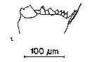 issued from : S.B. Schnack in Crustacean Issue, 1989, 6. [p.143, Fig.6, 1]. 1, Calocalanus pavo (from off NW Africa, upwelling region): Cutting edge of Md.
|
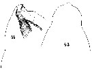 Issued from : W. Giesbrecht in Systematik und Faunistik der Pelagischen Copepoden des Golfes von Neapel und der angrenzenden Meeres-Abschnitte. – Fauna Flora Golf. Neapel, 1892, 19 , Atlas von 54 Tafeln. [Taf.36, Figs. 43, 44]. Female: 43, forehead (dorsal); 44, same (lateral).
|
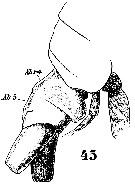 Issued from : W. Giesbrecht in Systematik und Faunistik der Pelagischen Copepoden des Golfes von Neapel und der angrenzenden Meeres-Abschnitte. – Fauna Flora Golf. Neapel, 1892, 19 , Atlas von 54 Tafeln. [Taf.36, Fig.45]. Female: 45, posterior part of thoracic segments and urosome (lateral).
|
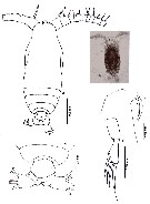 issued from : N. Phukham in Species diversity of calanoid copepods in Thai waters, Andaman Sea (Master of Science, Univ. Bangkok). 2008. [p.203, Fig.77]. Female (from W Malay Peninsula): a, habitus; b, forehead (lateral); c, urosome (dorsal); d, P5. Body length after drawing: F = 0.800 mm (caudal rami excluded).
|
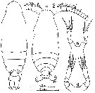 issued from : Mulyadi in Published by Res. Center Biol., Indonesia Inst. Sci. Bogor, 2004. [p.180, Fig.102]. Female (from Eastern Indonesian Seas): a, habitus (dorsal); b, P5. Immature female: c, habitus (dorsal); d, P5.
|
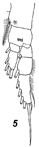 Issued from : V.N. Andronov in Russian Acad. Sci. P.P. Shirshov Inst. Oceanol. Atlantic Branch, Kaliningrad, 2014. [p.44, Fig.12, 5]. Calocalanus pavo after Andronov, 2014. Female P1.
|
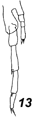 Issued from : V.N. Andronov in Russian Acad. Sci. P.P. Shirshov Inst. Oceanol. Atlantic Branch, Kaliningrad, 2014. [p.73, Fig.19: 13 ]. Calocalanus pavo after Andronov, 2014. Male P5.
| | | | | Ref. compl.: | | | Cleve, 1904 a (p.186); Pearson, 1906 (p.9); Rose, 1924 (p.10); 1925 (p.151); Wilson, 1942 a (p.173); Massuti Alzamora, 1942 (p.87); Oliveira, 1945 (p.191); Sewell, 1948 (p.357, 391, 395, 407, 414, 433, 439, 442, 450, 453, 456, 460, 463, 469, 477, 478, 481, 489, 493); C.B. Wilson, 1950 (p.179); Krishnaswamy, 1953 (p.116); Yamazi, 1958 (p.148, Rem.); Deevey, 1960 (p.5, Table II, annual abundance); Heinrich, 1960 (p.33); Fagetti, 1962 (p.12); Cervigon, 1962 (p.181, tables: abundance distribution); Ganapati & Shanthakumari, 1962 (p.7, 15); Grice & Hart, 1962 (p.287, table 3, table 4: abundance); Gaudy, 1962 (p.93, Rem.: p.104); Duran, 1963 (p.13); V.N. Greze, 1963 a (tabl.2); Shmeleva, 1963 (p.141); Gaudy, 1963 (p.21, Rem.); Björnberg, 1963 (p.29, Rem.); Unterüberbacher, 1964 (p.18); De Decker, 1964 (p.15, 18, 28); De Decker & Mombeck, 1964 (p.11); Pavlova, 1964 (p.1710); Roehr & Moore, 1965 (p.565, vertical distribution); Shmeleva, 1965 b (p.1350, lengths-volume -weight relation); Grice & Hulsemann, 1965 (p.223); Neto & Paiva, 1966 (p.21, Table III); Mazza, 1966 (p.69); 1967 (p.355: Rem.); Pavlova, 1966 (p.43); Ehrhardt, 1967 (p.737, 887, figs.51-53, geographic distribution), Rem.); Grice & Hulsemann, 1967 (p.14); Fleminger, 1967 a (tabl.1); Lubny-Gertzyk, 1968 (p.276); De Decker, 1968 (p.45); Delalo, 1968 (p.137); Evans, 1968 (p.11); Berdugo & Kimor, 1968 (p.447); Dowidar & El-Maghraby, 1970 (p.267); Itoh, 1970 a (tab.1); Park, 1970 (p.475); Salah, 1971 (p.319); Deevey, 1971 (p.224); Timonin, 1971 (p.281, trophic group); Carli, 1971 (p.372, tab.1); Binet & al., 1972 (p.73); Della Croce & al., 1972 (p.1, Rem.); Apostolopoulou, 1972 (p.327, 338, fig.1); Roe, 1972 (p.277, tabl.1, tabl.2); Bainbridge, 1972 (p.61, Appendix Table I: vertical distribution vs day/night, Table II: %, Table IV: seasonal abundance)); Guglielmo, 1973 (p.399); Heinrich, 1973 (p.95); Björnberg, 1973 (p.307, 384); Corral Estrada & Pereiro Muñoz, 1974 (tab.I); Patel, 1975 (p.659); Vives & al., 1975 (p.40, IV); Timonin, 1976 (p.79, vertical distribution); Madhu Pratap & al., 1977 (p.138, Table 3: abundance vs. stations); Deevey & Brooks, 1977 (p.256, tab.2, Station "S"); Tranter, 1977 (p.598); Carter, 1977 (1978) (p.35); Timonin & Voronina, 1977 (p.287, fig.5); Dessier, 1979 (p.201, 204); Porumb, 1980 (p.168); Vaissière & Séguin, 1980 (p.23, tab.2); Kovalev & Schmeleva, 1982 (p.83); Vives, 1982 (p.290); Brenning, 1982 (p.4, spatial distribution, T-S diagram, Rem.); Dessier, 1983 (p.89, Tableau 1, Rem., %); Turner & Dagg, 1983 (p.16); Tremblay & Anderson, 1984 (p.4); Guangshan & Honglin, 1984 (p.118, tab.); Tremblay & Anderson, 1984 (p.4, Rem.); De Decker, 1984 (p.315, 333: carte); Scotto di Carlo & al., 1984 (1043); Roe, 1984 (p.356); Cummings, 1984 (p.163, Table 2); Regner, 1985 (p.11, Rem.: p.24); Jansa, 1985 (p.108, Tabl.I, , II, III, IV, V); Brenning, 1985 a (p.23, Table 2); Almeida Prado Por, 1985 (p.250); Longhurst, 1985 (tab.2); Brinton & al., 1986 (p.228, Table 1); M. Lefèvre, 1986 (p.33); Madhupratap & Haridas, 1986 (p.105, tab.1); Renon, 1987 (tab.2); Jimenez-Perez & Lara-Lara, 1988; Lozano Soldevilla & al., 1988 (p.57); Dessier, 1988 (tabl.1); Suarez & al., 1990 (tab.2); Madhupratap & Haridas, 1990 (p.305, fig.6: vertical distribution night/day; fig.7: cluster); Othman & al., 1990 (p.561, 563, Table 1); Hirakawa & al., 1990 (tab.3); Yoo, 1991 (tab.1); Hattori, 1991 (tab.1, Appendix); Suarez & Gasca, 1991 (tab.2); McKinnon, 1991 (p.471); Suarez, 1992 (App.1); Seguin & al., 1993 (p.26, Rem.); Shih & Young, 1995 (p.71); Hajderi, 1995 (p.542); Madhupratap & al., 1996 (p.866); Padmavati & Goswami, 1996 a (p.85, fig.3, Table 4, vertical distribution); Kotani & al., 1996 (tab.2); Webber & al., 1996 (tab.1); Suarez-Morales & Gasca, 1997 (p.1525); Siokou-Frangou, 1997 (tab.1); Park & Choi, 1997 (Appendix); Hure & Krsinic, 1998 (p.100); Padmavati & al., 1998 (p.349); Gilabert & Moreno, 1998 (tab.1, 2); Alvarez-Cadena & al., 1998 (tab.1,2,3,4); Wong & al, 1998 (tab.2); Noda & al., 1998 (p.55, Table 3, occurrence); Mauchline, 1998 (tab.58); Suarez-Morales & Gasca, 1998 a (p108); Dolganova & al., 1999 (p.13, tab.1); Lavaniegos & Gonzalez-Navarro, 1999 (p.239, Appx.1); Neumann-Leitao & al., 1999 (p.153, tab.2); Razouls & al., 2000 (p.343, Appendix); Ueda & al., 2000 (tab.1); Sautour & al., 2000 (p.531, Table II, abundance); Fernandez-Alamo & al., 2000 (p.1139, Appendix); Lopez-Salgado & al., 2000 (tab.1); El-Sherif & Aboul Ezz, 2000 (p.61, Table 3: occurrence); Moraitou-Apostolopoulou & al., 2000 (tab.I, fig.7); Madhupratap & al., 2001 (p. 1345, vertical distribution vs. O2, figs.4, 5: clusters, Rem.: 1353); d'Elbée, 2001(tabl. 1); Holmes, 2001 (p.38); Lo & al., 2001 (1139, tab.I); Zerouali & Melhaoui, 2002 (p.91, Tableau I); Sameoto & al., 2002 (p.12); Dunbar & Webber, 2003 (tab.1); Vukanic, 2003 (139, tab.1); Hwang & al., 2003 (p.193, tab.2); Shimode & Shirayama, 2004 (tab.2); Hsiao & al., 2004 (p.326, tab.1); Rezai & al., 2004 (p.490, tab.2); Lo & al. *, 2004 (p.218, tab.1, fig.6); Lo & al., 2004 (p.468, tab.2); Chang & Fang, 2004 (p.456, tab.1); Vukanic & Vukanic, 2004 (p.9, tab. 2); Daly Yahia & al., 2004 (p.366, fig.4); Lan & al., 2004 (p.332, tab.1, tab.2); Satapoomin & al., 2004 (p.107, tab.4); Lo & al., 2004 (p.89, tab.1); Kazmi, 2004 (p.230); Smith & Madhupratap, 2005 (p.214, tab.6); Prusova & Smith, 2005 (p.75); Isari & al., 2006 (p.241, tab.II); Lopez-Ibarra & Palomares-Garcia, 2006 (p.63, Tabl. 1, seasonal abundance vs El-Niño, Rem.: p.70, 72); Araujo, 2006 (p.173, Tab.3): Lavaniegos & Jiménez-Pérez, 2006 (p.136, tab.2, 4, Rem.); Hwang & al., 2006 (p.943, tabl. I); Hooff & Peterson 2006 (p.2610); Hwang & al., 2007 (p.23); Dur & al., 2007 (p.197, Table IV); Fernandez de Puelles & al., 2007 (p.3340: fig.7); Valdés & al., 2007 (p.103: tab.1); Khelifi-Touhami & al., 2007 (p.327, Table 1); Jitlang & al., 2008 (p.65, Table 1); McKinnon & al., 2008 (p.844: Tab.I, p.848: Tab.IV); Neumann-Leitao & al., 2008 (p.799: Tab.II, fig.6); Rakhesh & al., 2008 (p.154, Table 5: abundance vs stations); Morales-Ramirez & Suarez-Morales, 2008 (p.518); Muelbert & al., 2008 (p.1662, Table 1); Ayon & al., 2008 (p.238, Table 4: Peruvian samples); Fernandes, 2008 (p.465, Tabl.2); Lan Y.C. & al., 2008 (p.61, Table 1, % vs stations, Table 2: indicator species); Tseng L.-C. & al., 2008 (p.153, Table 2, fig.5, occurrence vs geographic distribution, indicator species); Tseng & al., 2008 (p.402, Table 2); Pagano, 2009 (p.116); C.-Y. Lee & al., 2009 (p.151, Tab.2); Miyashita & al., 2009 (p.815, Tabl.II); Tseng & al., 2009 (p.327, fig.5, feeding); Lan Y.-C. & al., 2009 (p.1, Table 2, % vs hydrogaphic conditions); Brugnano & al., 2010 (p.312, Table 2, 3); Hernandez-Trujillo & al., 2010 (p.913, Table 2); Cornils & al., 2010 (p.2076, Table 3); Schnack-Schiel & al., 2010 (p.2064, Table 2: E Atlantic subtropical/tropical); Mazzocchi & Di Capua, 2010 (p.426); Fazeli & al., 2010 (p.153, Table 1); Medellin-Mora & Navas S., 2010 (p.265, Tab. 2); W.-B. Chang & al., 2010 (p.735, Table 2, 4, fig.5, abundance); Hsiao S.H. & al., 2011 (p.475, Appendix I); Maiphae & Sa-ardrit, 2011 (p.641, Table 2, 3, Rem.); Andersen N.G. & al., 2011 (p.71, Fig.3: abundance); Isari & al., 2011 (p.51, Table 2, abundance vs distribution); Pillai H.U.K. & al., 2011 (p.239, Table 3, vertical distribution); Selifonova, 2011 a (p.77, Table 1, alien species in Black Sea); Kâ & Hwang, 2011 (p.155, Table 3: occurrence %); Tseng L.-C. & al., 2011 (p.47, Table 2, occurrences vs mesh sizes); Hsiao & al., 2011 (p.317, Table 2, indicator of seasonal change); Shiganova & al., 2012 (p.61, Table 4); Uysal & Shmeleva, 2012 (p.909, Table I); Salah S. & al., 2012 (p.155, Tableau 1); Zizah & al., 2012 (p.79, Tabeau I, Rem.: p.86); Jang M.-C & al., 2012 (p.37, abundance and seasonal distribution); Mulyadi & Rumengan, 2012 (p.202, Rem.: p.204); Tseng & al., 2012 (p.621, Table 3: abundance); Lavaniegos & al., 2012 (p. 11, Appendix); Dorgham & al., 2012 (p.473, Table 3: abundance %); Takahashi M. & al., 2012 (p.393, Table 2, water type index); Gubanova & al., 2013 (in press, p.4, Table 2); Belmonte & al., 2013 (p.222, Table 2, abundance vs stations); Cornils & Blanco-Bercial, 2013 (p.861, Table 1, molecular analysis, figs.3, 4, 5); in CalCOFI regional list (MDO, Nov. 2013; M. Ohman, pers. comm.); Tseng & al., 2013 (p.507, seasonal abundance); Rakhesh & al., 2013 (p.7, Table 1, abundance vs stations); Lidvanov & al., 2013 (p.290, Table 2, % composition); Terbiyik Kurt & Polat, 2013 (p.1163, Table 2, seasonal distribution); Hwang & al., 2014 (p.43, Appendix A: seasonal abundance); Bonecker & a., 2014 (p.445, Table II: frequency, horizontal & vertical distributions); Zaafa & al., 2014 (p.67, Table I, occurrence); Zakaria, 2014 (p.3, Table 1, abundance vs 1960-2000); Mazzocchi & al., 2014 (p.64, Table 3, 4, 5, spatial & seasonal composition %); Dias & al., 2015 (p.483, Table 2, abundance, biomass, production); Zakaria & al., 2016 (p.1, Table 1, 3, 4); Benedetti & al., 2016 (p.159, Table I, fig.1, functional characters); Ben Ltaief & al., 2017 (p.1, Table III, Summer relative abundance); El Arraj & al., 2017 (p.272, table 2, spatial distribution); Marques-Rojas & Zoppi de Roa, 2017 (p.495, Table 1); Jerez-Guerrero & al., 2017 (p.1046, Table 1: temporal occurrence) ; Benedetti & al., 2018 (p.1, Fig.2: ecological functional group); Belmonte, 2018 (p.273, Table I: Italian zones); Abo-Taleb & Gharib, 2018 (p.139, Table 5, p.145: occurrence %); Chaouadi & Hafferssas, 2018 (p.913, Table II: occurrence); Palomares-Garcia & al., 2018 (p.178, fig.3: relative frequency, Table 1); Acha & al., 2020 (p.1, Table 3: occurrence % vs ecoregions). | | | | NZ: | 22 | | |
|
Carte de distribution de Calocalanus pavo par zones géographiques
|
| | | | | | | | | | | | | | | 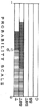 issued from : T.S.K. Björnberg in Bol. Inst. Oceanogr., Sao Paulo, 1963, XIII (1). [p.29, Fig.15]. issued from : T.S.K. Björnberg in Bol. Inst. Oceanogr., Sao Paulo, 1963, XIII (1). [p.29, Fig.15].
Probability of occurrence of Calocalanus pavo in different environments.
T: Tropical waters (above 36.00 p.1000 salinity and above 20°C temperature); SST: Surface subtropical waters (salinity around 36 p.1000 and temperature 18°C or less); DST: Deeper shelf waters (salinity between 34 and 36, temperature under 20°C p.1000); SS: Surface shelf waters (same salinity and temperature above 20°C);
C: coastal waters with low salinity and variable temperature.
In each column no shading means no probability of finding the species in the samples from this environment; horizontal shading indicates the probability of finding the sepecies in percentages less than one in samples from this environment; cross shading indicates the probability of finding it in percentages higher than one and black shading represents the probability of finding it in the largest percentages of the total number of copepods.
Nota: This species prefers waters of high salinities (above 36.00 p.1000) and high temperatures (above 25°C) off Brazil. It did not occur in deep waters. |
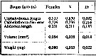 issued from : A.A. Shmeleva in Bull. Inst. Oceanogr., Monaco, 1965, 65 (n°1351). [Table 6: 11 ]. Calocalanus pavo (from South Adriatic). issued from : A.A. Shmeleva in Bull. Inst. Oceanogr., Monaco, 1965, 65 (n°1351). [Table 6: 11 ]. Calocalanus pavo (from South Adriatic).
Dimensions, volume and Weight wet. Means for 50-60 specimens. Volume and weight calculated by geometrical method. Assumed that the specific gravity of the Copepod body is equal to 1, then the volume will correspond to the weight. |
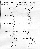 issued from : U. Brenning in Wiss. Z. Wilhelm-Pieck-Univ. Rostock - 31. Jahrgang 1982. Mat.-nat. wiss. Reihe, 6. [p.5, Fig.7]. issued from : U. Brenning in Wiss. Z. Wilhelm-Pieck-Univ. Rostock - 31. Jahrgang 1982. Mat.-nat. wiss. Reihe, 6. [p.5, Fig.7].
Spatial distribution for Calocalanus pavo, C. tenuis, C. styliremis, C. contractus from 8° S - 26° N; 16°- 20° W. |
 issued from : U. Brenning in Wiss. Z. Wilhelm-Pieck-Univ. Rostock - 31. Jahrgang 1982. Mat.-nat. wiss. Reihe, 6. [p.5, Figs.8]. issued from : U. Brenning in Wiss. Z. Wilhelm-Pieck-Univ. Rostock - 31. Jahrgang 1982. Mat.-nat. wiss. Reihe, 6. [p.5, Figs.8].
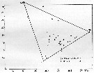
Spatial distribution for Calocalanus pavo, and C. tenuis from 8° S - 26° N; 16°- 20° W.
SO: Southern Surface Water (S °/oo: 34,50; T°C: 29,0); ND: Northern Water of the Surface Layer (S °/oo: 37,5; T°C: 21,0); SD: Southern Deep Water of the surface layer (S °/oo: 35,33; T°C: 13,4). See commentary in Temora stylifera and Brenning (1985 a, p.6).
Nota: This species is thermophile surface form. |
 Issued from : M. Madhupratap & P. Haridas in J. Plankton Res., 12 (2). [p.313, Fig.6]. Issued from : M. Madhupratap & P. Haridas in J. Plankton Res., 12 (2). [p.313, Fig.6].
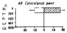
Vertical distribution of calanoid copepod (mean +1 SE), abundance No/100 m3. 69- Calocalanus pavo.
Night: shaded, day: unshaded.
Samples collected from 6 stations located off Cochin (India), SE Arabian Sea, November 1983, with a Multiple Closing Plankton Net (mesh aperture 300 µm), in vertical hauls at 4 depth intervalls (0-200, 200-400, 400-600, 600-1000 m). |
| | | | Loc: | | | Cosmopolite (tropical, sub-tropical): sub-Antarct. (Indian), South Africa (E & W), Angola (Baia Farta), G. of Guinea, off Lagos, Senegal-Mauritania, Uruguay (continental shelf), Brazil (S, Campos Basin, off Natal), Caribbean Colombia, Bahia de Mochima (Venezuela), Cariaco Basin, Yucatan, G. of Mexico, Jamaica, Straits of Florida, Florida, Sargasso Sea, off Bermuda, Station "S" (32°10'N, 64°30'W), Delaware Bay (outside), off Woods-Hole, off E Nova Scotia, off SW Ireland, Canary Is., Morocco-Mauritania, Cap Ghir, Moroccan copast, Bay of Biscay, Ibero-moroccan Bay, off W Tangier, Medit. (M'Diq, Alboran Sea, Habibas Is., Sidi fredj coast, Algiers, N Tunisia, Castellon, Baleares, Banyuls, G. of Lion, Marseille, Monaco, Genova, Tyrrhenian Sea, Milazzo, Strait of Messina, G. of Gabes, Taranto, Malta, Adriatic Sea, Ionian Sea, Aegean Sea, Thracian Sea, W Egyptian coast, Iskenderun Bay, Lebanon Basin, Alexandria, Marmara Sea, Black Sea), off Sharm El-Sheikh, G. of Aqaba (Taba), Hurghada, Red Sea, Gulf of Oman, G. of Aden, Arabian Sea, Maldive Is., Natal, Madagascar, Seychelles, Indian, India (Saurashtra coast, Goa - Gujarat, Sri Lanka, Madras, Godavarizone, Kakinada Bay), Bay of Bengal, Barren Island, S Burma, Nicobar Is., off Phuket, W Malay Peninsula (Andaman Sea), Straits of Malacca, G. of Thailand, Indonesia: Lombok Sea, Flores Sea, SW Sulawesi, Ceram Is. (Ambon Bay), S Celebes Sea, China Seas (Yellow Sea, East China Sea, South China Sea), Taiwan Strait, Taiwan (S, E, SW, W, Tapong Bay, Kaohsiung Harbor, NW, N, Mienhua Canyon, NE), Korea, Korea Strait, Japan Sea, Japan, Kuchinoerabu Is., off Sanriku, Pacif. E (equatorial), off Washington & Oregon coasts, Baja California (Bahia Magdalena, W), G. of California, La Paz, G. of Tehuantepec, off Guatemala W, W Costa Rica, Clipperton Is., Pacif. (W equatorial), Australia (G. of Carpentaria, North West Cape, Great Barrier), New Caledonia, Bering Sea, off Kamchatka,Bahia Cupica (Colombia), Galapagos-Ecuador, Peru, N Chile
Data from Cornils & Blanco-Bercial (2013): 05°07'S; 119°21'E. | | | | N: | 377 | | | | Lg.: | | | (14) F: 1,21-0,9; (28) F: 0,9; (34) F: 1,15; (45) F: 1,25-0,8; M: 1,15-1; (47) F: 1,2-0,88; M: 1,04; (55) F: 1,23; (66) F: 0,91-0,79; (72) F: 1,18-1,05; (73) F: 1,06-0,95; (75) F: 0,92; (91) F: 1,4-0,85; (101) F: 1,19-0,85; (114) F: 1,1; (150) F: 1,35-1,12; (180) F: 1,22-0,98; M: 0,95-0,91; (187) F: 1,5-1,38; (188) F: 1,2-0,88; M: 1,04; (199) F: 1,29-1,06; (202) F: 0,88-1,22; M: 0,91-1,01; (237) F: 1,2-0,65; (290) F: 1,25-1; (333) F: 1,12-0,9; (334) F: 1,2-0,88; M: 1,04; (335) F: 0,94-0,91; M: 0,92-0,88; (338) M: 1,05-0,63; (432) F: 1,2-0,9; (449) F: 1,22-0,88; M: 1,04; (530) F: 1; (785) F: 0,88-0,83; (786) F: 1,05-0,94; (795) F: 0,86; (866) F: 0,9-1,3; M: 0,6-1,1; (920) F: 1,05; (991) F: 0,85-1,4; M: 1,04-1,18; (1023) F: 0,96-1,00; (1112) F: 0,864-1,28; (1122) F: 1,1; (1132) F: 0,98-1,2; M: 1,04; {F: 0,65-1,50; M: 0,60-1,18} | | | | Rem.: | Epipélagique, parfois plus profonde.
Sampling depth (sub-Antarct.) : 0-100 m.
Voir aussi les remarques en anglais | | | Dernière mise à jour : 25/10/2022 | |
|
|
 Toute utilisation de ce site pour une publication sera mentionnée avec la référence suivante : Toute utilisation de ce site pour une publication sera mentionnée avec la référence suivante :
Razouls C., Desreumaux N., Kouwenberg J. et de Bovée F., 2005-2026. - Biodiversité des Copépodes planctoniques marins (morphologie, répartition géographique et données biologiques). Sorbonne Université, CNRS. Disponible sur http://copepodes.obs-banyuls.fr [Accédé le 22 mai 2026] © copyright 2005-2026 Sorbonne Université, CNRS
|
|
|
|




;)
;)
;)
;)
;)
;)
;)
;)
;)
;)
;)
;)
;)
;)
;)
;)
;)
;)
;)
;)
;)

;)
;)
;)
;)
;)