|
|
 |
Fiche d'espèce de Copépode |
|
|
Calanoida ( Ordre ) |
|
|
|
Eucalanoidea ( Superfamille ) |
|
|
|
Rhincalanidae ( Famille ) |
|
|
|
Rhincalanus ( Genre ) |
|
|
| |
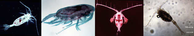
Rhincalanus nasutus Giesbrecht, 1888 (F,M) | |
| | | | | | | Syn.: | Rhincalanus gigas : T. Scott,1901; A. Scott, 1909 (p.24, Rem.); Sewell, 1914 a (p.204, Rem.);
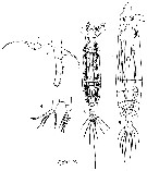
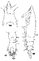
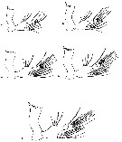
Eucalanus nasutus Sars, 1912 (p.654); Massuti Alzamora, 1942 (p.110); Baessa De Aguiar, 1991 (1993) (p.106); | | | | Ref.: | | | Giesbrecht, 1892 (p.152, 160, figs.F,M); Giesbrecht & Schmeil, 1898 (p.22); Sars, 1901 a (1903) (p.15, figs.F); Thompson & Scott, 1903 (p.233, 242); Esterly, 1905 (p.136, figs.F); Farran, 1908 b (p.22); Wolfenden, 1911 (p.194); With, 1915 (p.44, figs.F,M); Willey, 1918 (1919) (p.186, figs. juv.); Lysholm & Nordgaard, 1921 (p.9); Sars, 1925 (p.23); Farran, 1926 (p.232); Sewell, 1929 (p.58, 60, fig.F, Rem.); Rose, 1929 (p.15); Farran, 1929 (p.208, 220); Sewell, 1929 (p.58, fig.); Sciacchinato, 1930 (p.9, figs.F); Wilson, 1932 a (p.34, figs.F,M); Dakin & Colefax, 1933 (p.204); Jespersen, 1934 (p.47, fig.11); Tanaka, 1935 (p.151, figs.F,M); Farran, 1936 a (p.79); Gibbons, 1936 (p.385, figs. Nauplii); Mori, 1937 (1964) (p.26, figs.F,M); Dakin & Colefax, 1940 (p.95, figs.F,M); Jespersen, 1940 (p.13, fig.3); Wilson, 1942 a (p.205, fig.F); Pesta, 1943 (p.12, figs.F,M); Vervoort, 1946 (p.122, Rem.); Sewell, 1947 (p.49, Rem.); Brodsky, 1950 (1967) (p.107, figs.F,M); Farran & Vervoort, 1951 b (n°34, p.3, figs.F,M); Marques, 1953 (p.95, figs.F, M juv.); Tanaka, 1956 (p.271); Vervoort, 1957 (p.33, Rem.); Marques, 1959 (p.207); Ganapati & Shanthakumari, 1962 (p.7, 16); Fagetti, 1962 (p.10); Grice, 1962 (p.183); Vervoort, 1963 b (p.101); Mazza, 1962 (p.332, figs.F); Chen & Zhang, 1965 (p.38, figs.F); Saraswathy, 1966 (1967) (p.75); Owre & Foyo, 1967 (p.37, figs.F,M); Mazza, 1967 (p.89, figs.F,M, juv.); Marques, 1968 a (p.396); Vinogradov, 1968 (1970) (p.268, 277); Vilela, 1968 (p.10, figs.F); Ramirez, 1969 (p.49, figs.F, Rem.); Corral Estrada, 1970 (p.82); Minoda, 1971 (p.18); Bradford, 1972 (p.34, figs.F, juv.M); Razouls, 1972 (p.94, Annexe: p.13, figs.F,M); Vives & al., 1975 (p.35, tab.II); Goswami & Goswami, 1979 (p.103, figs.); Dawson & Knatz, 1980 (p.4, figs.F,M); Björnberg & al., 1981 (p.621, figs.F,M); Gardner & Szabo, 1982 (p.160, figs.F,M); Schnack, 1982 (p.145, fig.Md); Brodsky & al., 1983 (p.202, figs.F,M, Rem.); Roe, 1984 (p.356); Sazhina, 1985 (p.38, figs. N); Baessa de Aguiar, 1986 (1989) (p.59, Rem.); Zheng Zhong & al., 1989 (p.230, figs.F,M); Schnack, 1989 (p.137, tab.1, fig.6: Md); Huys & Boxshall, 1991 (p.66, fig.); Bradford-Grieve, 1994 (p.85, figs.F,M, fig. 100); Mazzocchi & al., 1995 (p.125, figs.F, Rem.); Chihara & Murano, 1997 (p.787, Pl.96: F,M); Hure & Krsinic, 1998 (p.20, 100); Lapernat, 1999 (p.16, 55); Bradford-Grieve & al., 1999 (p.878, 912, figs.F,M); Conway & al., 2003 (p.170, figs.F,M, Rem.); Goetze, 2003 (p.2322 & suiv.); G. Harding, 2004 (p.39, figs.F,M); Boxshall & Halsey, 2004 (p.176; p.177: figs.F); Mulyadi, 2004 (p.122, figs.F,M, Rem.); Vives & Shmeleva, 2007 (p.886, figs.F,M, Rem.) ; Hidalgo & al., 2012 (p.1025, stages N, copepodis 1-5: figs.3-18); Andronov, 2014 (p.36, fig.: A2) | 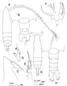 issued from : J.M. Bradford-Grieve in The Marine Fauna of New Zealand: Pelagic Calanoid Copepoda. National Institute of Water and Atmospheric Research (NIWA). New Zealand Oceanographic Institute Memoir, 102, 1994. [p.86, Fig.46]. Female: A, habitus (dorsal); B, urosome (dorsal); C, forehead (lateral right side); D, Md (mandibular palp); E, P1; F, P5. Male: G, habitus (dorsal); H, urosome (dorsal); I, P5. There appear to be some differences between Giesbrecht's (1892) figures and the Southwest Pacific specimens.
|
 issued from : G.O. Sars in An Account of the Crustacea of Norway. Vol. IV. Copepoda Calanoida. Published by the Bergen Museum, 1903. [Pl. VI]. Female. C = forehead (ventral wiew and lateral left side).
|
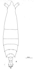 Issued from: M.G. Mazzocchi, G. Zagami, A. Ianora, L. Guglielmo & J. Hure in Atlas of Marine Zooplankton Straits of Magellan. Copepods. L. Guglielmo & A. Ianora (Eds.), 1995. [p.126, Fig.3.20.1]. Female: A, habitus (dorsal). Nota: Head clearly separated from the 1st thoracic somite. Caudal rami slightly asymmetrical bearing 2 tufts of hairs of anal region. Two large spines visible on dorsal side of genital somite. The3-segmented abdomen is due to fusion of the anal somite with the furca.
|
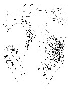
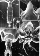 &Issued from: M.G. Mazzocchi, G. Zagami, A. Ianora, L. Guglielmo & J. Hure in Atlas of Marine Zooplankton Straits of Magellan. Copepods. L. Guglielmo A. Ianora (Eds.), 1995. [p.127, Fig.3.20.2]. Female (SEM preparation): A, habitus (dorsal); B, forehead (dorsal); C, forehead with rostral filaments (ventral); D, 4th thoracic somite and urosome (dorsal); E, anal region bearing tufts of hairs on ventral surface; F, P5. Bars: A 1 mm; B-F 0.100 mm.
|
 issued from : G.O. Sars in An Account of the Crustacea of Norway. Vol. IV. Copepoda Calanoida. Published by the Bergen Museum, 1903. [Pl.VII]. Female. L = labrum; l = labium (paragnathes). Nota: For Boxshall & Halsey (2004, p.176) P5 is re-interpreted as a transverse plate formed by coxae and intercoxal sclerite, a separate basis and a 1-segmented exopod. For the authors the evidence for this re-interpretation is the presence of an inner element on the proximal free segment (the inner seta on the 1st exopodal segment is lost in the vast majority of calanoids, being retained only in a few members of basal families, such as the Epactriscidae); the inner element is more likely a vestige of the endopod, identifying that segment as the basis.
|
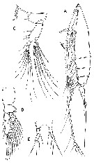
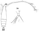 issued from : F.C. Ramirez in Contr. Inst. Biol. mar., Buenos Aires, 1969, 98. [p.50, Lam. VIII, figs.46, 54]. Female (from off Mar del Plata): 46, habitus (dorsal); 54, P5. Scale bars in mm: 1.5 (46); 0.05 (54).
|
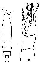
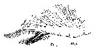
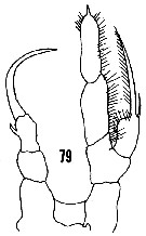
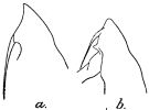 issued from : R.B.S. Sewell in Mem. Indian Mus., 1929, X. [p.59, Fig.19]. From off SE Sri Lanka: a, forehead (lateral); b, idem in Rhincalanus gigas (from South Ocean).
|
 issued from : R.B.S. Sewell in Mem. Indian Mus., 1929, X. [p.60]. Main points of difference between R. gigas and R. nasutus.
|
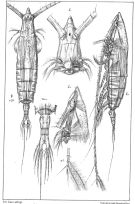
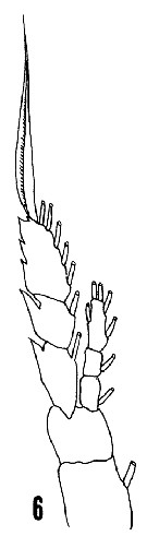
 issued from : T. Mori in The pelagic Copepoda from the neighbouring waters of Japan, 1937 (2nd edit., 1964). [Pl.10, Figs.6-9]. Female: 6, P5; 9, habitus (dorsal). Male: 7, P5; 8, habitus (dorsal).
|
 issued from : C.O. Esterly in Univ. Calif. Publs Zool., 1905, 2 (4). [p.136, Fig.10]. Female (from San Diego Region): a, habitus (dorsal); b, P5.
|
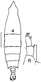 issued from : J.M. Bradford in Mem. N. Z. Oceonogr. Inst., 1972, 54. [p.35, Fig.5 (4, 6)]. Female (from Kaikoura, New Zealand): 4, habitus (dorsal); 6, P5. Scale bars: 1 mm (4); 0.1 mm (6).
|
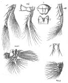
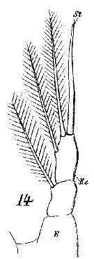
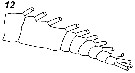
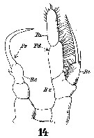 Issued from : W. Giesbrecht in Systematik und Faunistik der Pelagischen Copepoden des Golfes von Neapel und der angrenzenden Meeres-Abschnitte. - Fauna Flora Golf. Neapel, 1892, 19 , Atlas von 54 Tafeln. [Taf.9, Fig.14]. Male: 14, P5 (anterior view). Ps = left leg; Pd = right leg; B2 = basis; Re = exopod.
|
 Issued from : W. Giesbrecht in Systematik und Faunistik der Pelagischen Copepoden des Golfes von Neapel und der angrenzenden Meeres-Abschnitte. - Fauna Flora Golf. Neapel, 1892, 19 , Atlas von 54 Tafeln. [Taf.9, Fig.6]. Female: 6, A1 (proximal segments 1-14; ventral view).
|
 Issued from : W. Giesbrecht in Systematik und Faunistik der Pelagischen Copepoden des Golfes von Neapel und der angrenzenden Meeres-Abschnitte. - Fauna Flora Golf. Neapel, 1892, 19 , Atlas von 54 Tafeln. [Taf.9, Fig.6]. Female: 6, A1 'distal segments 14-25; ventral view).
|
 Issued from : W. Giesbrecht in Systematik und Faunistik der Pelagischen Copepoden des Golfes von Neapel und der angrenzenden Meeres-Abschnitte. - Fauna Flora Golf. Neapel, 1892, 19 , Atlas von 54 Tafeln. [Taf.35, Figs.46, 47, 49]. Female: 46, head (ventral); 47, urosome (ventral); 49, habitus (lateral).
|
 issued from : R. Huys & G.A. Boxshall in Copepod Evolution. The Ray Society, 1991, 159. [p.66, Fig.2.2.13, D]. Female (from Terra Nova Expedition 1910, Stns 80-120): D, A2.
|
 issued from : R. Huys & G.A. Boxshall in Copepod Evolution. The Ray Society, 1991, 159. [p.75, Fig.2.2.22, D]. D, endopod of Mxp.
|
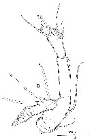
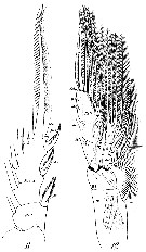
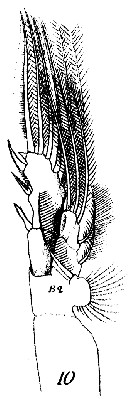
 Issued from : W. Giesbrecht in Systematik und Faunistik der Pelagischen Copepoden des Golfes von Neapel und der angrenzenden Meeres-Abschnitte. - Fauna Flora Golf. Neapel, 1892, 19 , Atlas von 54 Tafeln. [Taf.12, Figs.9, 16, 17]. Female: 9, Md (palp; posterior view); 16, Mxp (anterior surface); 17, A2 (anterior surface).
|
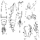
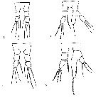
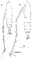 issued from : C. Razouls in Th. Doc. Etat Fac. Sc. Paris VI, 1972, Annexe. [Fig.25, A-B]. Female (from Banyuls, G. of Lion): B, habitus (dorsal). Male: A, habitus (dorsal).
|
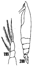 issued from : H.B. Owre & M. Foyo in Fauna Caribaea, 1, Crustacea, 1: Copepoda. Copepods of the Florida Current. [p.38, Figs.199, 200]. Redrawn after Giesbrecht, 1892. Female: 199, P5; 200, habitus (lateral). Nota:Forehead with a conical projection, rostral filaments not visible in dorsal view. P5 with 1 seta on the 2nd segment and 3 on the 3rd.
|
 issued from : H.B. Owre & M. Foyo in Fauna Caribaea, 1, Crustacea, 1: Copepoda. Copepods of the Florida Current, 1967. [p.11, Fig.6]. Female: 6, P4.
|
 issued from : H.B. Owre & M. Foyo in Fauna Caribaea, 1, Crustacea, 1: Copepoda. Copepods of the Florida Current, 1967. [p.21, Fig.79]. After Giesbrecht, 1892. Male: 79, P5. Nota: P5 terminates in a strongly curved seta.
|
 issued from : K.A. Brodsky, N.V. Vyshkvartseva, M.S. Kos & E.L. Markhaseva in Opred. Fauna SSSR., 1983, 1. [p.203, Fig.91]. After Mori, 1937; Giesbrecht, 1892. Female & Male. L: left leg; R: right leg.
|
 issued from : G.A. Boxshall & S.H. Halsey in An introduction to copepod diversity. The Ray Society, 2004, 166. [p.177, Fig.41]. Redrawn from Sars (1901). Female: A, habitus (lateral); C, Md; D, P1; E, P5. Nota: 3rd and 4thpedigerous somites each with paired spinous processes dorsally on posterior margin.
|
 Issued from : W. Giesbrecht in Systematik und Faunistik der Pelagischen Copepoden des Golfes von Neapel und der angrenzenden Meeres-Abschnitte. - Fauna Flora Golf. Neapel, 1892, 19 , Atlas von 54 Tafeln. [Taf.12, Figs.11, 12]. Female: 11, exopod of P1; 12, P4 (anterior surface).
|
 Issued from : W. Giesbrecht in Systematik und Faunistik der Pelagischen Copepoden des Golfes von Neapel und der angrenzenden Meeres-Abschnitte. - Fauna Flora Golf. Neapel, 1892, 19 , Atlas von 54 Tafeln. [Taf.12, Figs.10]. Female: 10, P1 (anterior surface).
|
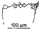 issued from : S.B. Schnack in Crustacean Issue, 1989, 6. [p.143, Fig.6: 7]. 7, Rhincalanus nasutus (from off NW Africa, upwelling region): Cutting edge of Md.
|
 Issued from : W. Giesbrecht in Systematik und Faunistik der Pelagischen Copepoden des Golfes von Neapel und der angrenzenden Meeres-Abschnitte. Fauna Flora Golf. Neapel, 1892, 19 , Atlas von 54 Tafeln. [Taf.12, Fig.14]. Female: 14, P5.
|
 issued from : Mulyadi in Published by Res. Center Biol., Indonesia Inst. Sci. Bogor, 2004. [p.122, Fig.70]. Female (from Indonesian Seas): a, habitus (dorsal); b-c, forehead (lateral and ventral, respectively); d, last thoracic segment and urosome (lateral right side); e, P5. Male: f, habitus (dorsal); g, P5.
|
 Issued from : V.N. Andronov in Russian Acad. Sci. P.P. Shirshov Inst. Oceanol. Atlantic Branch, Kaliningrad, 2014. [p.36, Fig.9, 12]. Rhincalanus nasutus after Sars, 1903. 12, Exopod of A2.
|
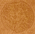 Issued from : P. Hidalgo, F. Ferrari, S. Yañez, P. Pino & R. Escribano in Crustaceana, 2012, 85 (9). [p.1030, Fig.2]. From off Conception (central-southern Chile). Photograph of normal eggs of Rhincalanus nasutus (Giesbrecht, 1888). Published in colour in the online edition (http://booksandjournals. brillonline.com/content/15685403). Nota: Eggs well-rounded with a dense pigmentation and yellowish colouration; under a compound microscope, their external membrane appears thin. Mean egg diameter 202 µm (n = 367) and ranged between 196 and 222 µm.
|
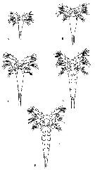 Issued from : P. Hidalgo, F. Ferrari, S. Yañez, P. Pino & R. Escribano in Crustaceana, 2012, 85 (9). [p.1031, Fig.3]. Ventral view of naupliar stages of Rhincalanus nasutus (Giesbrecht, 1888). A: Naulius 2; B: Nauplius 3; C: Nauplus 4; D: Nauplus 5; E: Nauplius 6. Nota: For this species, only naupius 2 and 5 have been described previously although there has been some confusion about the identity of tyhese stages (Gurney, 1934; Steuer, 1935). Nauplius 2: Average body length 0.44 mm (0.41-0.49, n = 109). Nauplius 3: Average body length 0.69 mm (0.66-0.71, n = 50). Nauplius 4: Average body length 0.89 mm (0.88-0.90, n = 12). Nauplius 5: Average body length 1.11 mm (1.10-1.13, n = 35). Nauplius 6: Average body length 1.33 mm (1.29-1.35, n = 11).
|
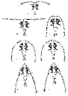 ssued from : P. Hidalgo, F. Ferrari, S. Yañez, P. Pino & R. Escribano in Crustaceana, 2012, 85 (9). [p.1037, Fig.7]. Ventral view of copepodid stages of Rhincalanus nasutus (Giesbrecht, 1888). A: C I; B: C II; D: C III; D: C IV female; E: C IV male; F: C V female; G: C V male. Nota: Copepodids elongate, with transparent body; head pointed dorsally and laterally; rostrum distinctly pointed; caudal ramus with 3 terminal setae and 2 long setae on the lateral edge. Copepodid I: Body length 1.6-1.8 mm (n = 85). A1 10-segmented (12 on the figure 8A). Copepodid II: Body length 1.7-2.1 mm (n = 290). A1 17-segmented (16 on the figure 8B) Copepodid III: Body length 2.2-2.6 mm (n = 152). A1 21-segmented (23 on the figure 8C). Copepodid IV female: Body length 3.2-3.9 mm (n =65). A1 23-segmented. Copepodid IV male: Body length 3.0-3.7mm (n = 29). Copepodid V female: Body length 3.9-4.2 mm (n = 21). A1 23-segmented. Copepodid V male: Body length 4.2-4.7 mm (n = 70).
|
 ssued from : P. Hidalgo, F. Ferrari, S. Yañez, P. Pino & R. Escribano in Crustaceana, 2012, 85 (9). [p.1040, Fig.10]. Mandible of copepodid stages of Rhincalanus nasutus (Giesbrecht, 1888). A; C I; B: C II; C: C III; D: C IV; E: C V. Nota Fig.10A: Md 2-segmented protopod; coxa with well-developed toothed gnathobase with proximal seta; basipod with 4 medial setae. Endopod 2-segmented with 1 and 4 setae. Exopod 5-segmented with 1, 1, 1, 1, 2 setae
|
 ssued from : P. Hidalgo, F. Ferrari, S. Yañez, P. Pino & R. Escribano in Crustaceana, 2012, 85 (9). [p.1050, Fig.18]. Swimming legs 5 of copepodid stages of Rhincalanus nasutus (Giesbrecht, 1888). A: C IV female; B: C IV male; C: C V female; D: C V male.
|
 ssued from : P. Hidalgo, F. Ferrari, S. Yañez, P. Pino & R. Escribano in Crustaceana, 2012, 85 (9). [p.1036, Table 3]. Summary of the morphometric characteristics (means) of the copepodid stages of Rhincalanus nasutus (Giesbrecht, 1888), obtained from the central-southern Chile.
| | | | | Ref. compl.: | | | Cleve, 1904 a (p.196, as Rhinocalanus nasutus); Pearson, 1906 (p.8, Rem.); Rose, 1925 (p.151); Wilson, 1932 (p.32); Hardy & Gunther, 1935 (1936) (p.147, Rem.); Jespersen, 1939 (p.40); Lysholm & al., 1945 (p.9); Oliveira, 1945 (p.191); C.B. Wilson, 1950 (p.318); Østvedt, 1955 (p.14: Table 3, p.55); Kott, 1957 (p.6, 17); Yamazi, 1958 (p.147, Rem.); Conover, 1960 (p.399, Table I, respiratory rate); Deevey, 1960 (p.5, Table II, annual abundance) ; Fish, 1962 (p.9); Marshall & Orr, 1962 (tab.3); Gaudy, 1962 (p.93, 99, Rem.: p.102); Duran, 1963 (p.13); Giron-Reguer, 1963 (p.27); Gaudy, 1963 (p.20, Rem.); Ahlstrom & Thrailkill, 1963 (p.57, Table 5, abundance);Björnberg, 1963 (p.24, Rem.); Shmeleva, 1964 a (p.1068); Unterüberbacher, 1964 (p.15, Rem.); De Decker, 1964 (p.16, 24, 29); Grice & Hulsemann, 1965 (p.223); Shmeleva, 1965 b (p.1350, lengths-volume -weight relation); Furuhashi, 1966 a (p.295, vertical distribution vs mixing Oyashio/Kuroshio region); Mullin, 1966 (p.546, Table I, III, diet); Neto & Paiva, 1966 (p.20, Table III); Mazza, 1966 (p.69); 1967 (p.367); Ehrhardt, 1967 (p.737, geographic distribution), Rem.); Mullin & Brooks, 1967 (p.657, life history, fecondity, growth-feeding); Grice & Hulsemann, 1967 (p.14); Fleminger, 1967 a (tabl.1); Matthews, 1967 (p.159, Table 1, Rem.); De Decker, 1968 (p.45); Delalo, 1968 (p.137); Omori, 1969 (p.5, Table 1); Itoh, 1970 a (p.1, tab.2); Morris, 1970 (p.2300, 2302); Lee & al., 1971 (p.1150); Shih & al., 1971 (p.39, 147); Gamulin, 1971 (p.382, tab.3); Deevey, 1971 (p.224); Gueredrat, 1971 (p.300, fig.2, 10, Table 1, 2); Brodsky, 1972 (P.256); Roe, 1972 (p.277, tabl.1, tabl.2); 1972 a (p.327); Boucher & Thiriot, 1972 (p.47, Tableau 4); Subbaraju & Krishnamurphy, 1972 (p.25, 26 ); Heinrich, 1973 (p.95); Björnberg, 1973 (p.300, 389); Harding, 1974 (p.141, tab.2, gut contents); Corral Estrada & Pereiro Muñoz, 1974 (tab.I); Nival & al., 1974 (p.231, respiration & excrétion); Peterson & Miller, 1975 (p.642, 650, Table 3); Patel, 1975 (p.659); Boucher & al., 1975 (p.85, nutrition/enzyme); Arashkevich, 1975 (p.351, digestion time); Vives & al.: 1975 (p.35, tab.II, III, IV); Arcos, 1976 (p.85, Rem.: p.91, Table II); Peterson & Miller, 1976 (p.14, Table 1, 2, 3, abundance vs interannual variations); Deevey & Brooks, 1977 (p.256, Table 2, Station "S"); Grindley, 1977 (p.341, Table 2); Peterson & Miller, 1977 (p.717, Table 1, seasonal occurrence); Timonin & Voronina, 1977 (p.286); Carter, 1977 (1978) (p.35); Stephen & Iyer, 1979 (p.228, tab.1, 3, 4, figs.3, 4); Pipe & Coombs, 1980 (p.223, vertical occurrence); Vaissière & Séguin, 1980 (p.23, tab.1); Svetlichnyi, 1980 (p.28, Table 1, passive submersion); Sreekmaran Nair & al., 1981 (p.493, Fig.2 cont.); Shadrin & Mel'nik, 1981 (p.82, population abundance vs. food intake); Rudyakov, 1982 (p.208, Table 2); Kovalev & Shmeleva, 1982 (p.82); Vives, 1982 (p.290); Smith S.L., 1982 (p.1347, Table 5, grazing); Turner & Dagg, 1983 (p.16, 22); Landry, 1983 (p.614, development times vs. stages); Minkina, 1983 (p.38, speed swimming); Dessier, 1983 (p.89, Tableau 1, Rem., %); Scotto di Carlo & Ianora, 1983 (p.150); Scotto di Carlo & al., 1984 (p.1044); Pieper & Holliday, 1984 (p.226, Table 1, Figs.3, 7, 8); De Decker, 1984 (p.315, 362: chart); Tremblay & Anderson, 1984 (p.5); Sameoto, 1984 (p.767, vertical migration); Longhurst, 1985 (tab.2); Brenning, 1985 a (p.24, Table 2); Baars & Oosterhuis, 1985 (p.71, Table 4: gut passage time); Brinton & al., 1986 (p.228, Table 1); Fleminger, 1986 (p.84, figs. 3, 4, Rem.); Chen Y.-Q., 1986 (p.205, Table 1: abundance %, fig.6, Table 2: vertical distribution); Wishner & Allison, 1986 (tab.2); Madhupratap & Haridas, 1986 (p.105, tab.1); Hakanson, 1987 (p.881, lipid content); Cowles & al., 1987 (p.653, fig.7, ingestion); Lozano Soldevilla & al., 1988 (p.57); Jimenez-Perez & Lara-Lara, 1988; Wiebe & al., 1988 (tab.7); Ohman, 1988 (p.143, Table 1: lipid content); Cervantes-Duarte & Hernandez-Trujillo, 1989 (tab.3); Echelman & Fishelson, 1990 a (tab.2 as Rhinocalanus); Heinrich, 1990 (p.16); Timonin, 1990 (p.479); Hirakawa & al., 1990 (tab.3); Madhupratap & Haridas, 1990 (p.305, fig.6: vertical distribution night/day; fig.7: cluster); Peterson & al., 1990 (p.259, Table 1, feeding); Suarez & al., 1990 (tab.2); Baars & al., 1990 (p.538: Rem.); Arinardi, 1991 (p.295); Fransz & al., 1991 (p.9); Santos & Ramirez, 1991 (p.79); Hattori, 1991 (tab.1, Appendix); Shih & Marhue, 1991 (tab.3); Scotto di Carlo & al., 1991 (p.271); Suarez & Gasca, 1991 (tab.2); Morales C.E. & al., 1991 (p.455, Table I, grazing); Mullin, 1991 a (p.1381, reproduction & mortality variability); Hernandez-Trujillo, 1991 (1993) (tab.I); Suarez, 1992 (App.1); Heinrich, 1992 (p.86); Huntley & Lopez, 1992 (p.201, Table A1, B1, egg-adult weight, temperature-dependent production, growth rate); Ayukai & Hattori, 1992 (p.163, Table 5, fecal pellet production rate); Jiyalal Ram & Goswami, 1993 (p.129, tab.IV); Ashjian & Wishner, 1993 (p.483, abundance, species group distributions); Seguin & al., 1993 (p.23); Hays & al., 1994 (tab.1); Landry & al., 1994 (p.55, abundance, grazing); Farstey, 1994; Palomares Garcia & Vera, 1995 (tab.1); Shih & Young, 1995 (p.70); Hirakawa & al., 1995 (tab.2); Errhif & al., 1997 (p.422); Timonin, 1997 (p.83, Rem.); Park & Choi, 1997 (Appendix); Padmavati & al., 1998 (p.349); Noda & al., 1998 (p.55, Table 3, occurrence); Weslawski & Legezynska, 1998 (p.1238); Gilabert & Moreno, 1998 (tab.1, 2); Suarez-Morales, 1998 (p.345, Table 1); Suarez-Morales & Gasca, 1998 a (p.109); Ohman & al., 1998 (p.1709, organic composition, vertical distribution, ETS activity, egg production, dormancy: Table3); Verheye & al., 1998 (p.317, Table II); Mauchline, 1998 (tab.8, 21, 23, 33, 35, 46, 47, 63, 64, 65); Reid & Hunt, 1998 (p.310, figs.2, 3, Rem.); Smith S. & al., 1998 (p.2369, Table 6, moonsoon effects); Barange & al., 1998 (p.1663, Table 2, abundance vs STC region); Hernandez-Trujillo, 1999 (p.284, tab.1); Lavaniegos & Gonzalez-Navarro, 1999 (p.239, Appx.1); Corten, 1999 (p.191, Table 1, fig.3); Lapernat, 2000 (tabl.3, 4); Razouls & al., 2000 (p.343, Appendix); Fernandez-Alamo & al., 2000 (p.1139, Appendix); Pakhomov & al., 2000 (p.1663, Table 2, transect Cape Town-SANAE antarctic base); Suarez-Morales & al., 2000 (p.751, tab.1); Seridji & Hafferssas, 2000 (tab.1); Madhupratap & al., 2001 (p. 1345, vertical distribution vs. O2, figs.4, 5: clusters); d'Elbée, 2001 (tabl. 1); Hidalgo & Escribano, 2001 (p.159, tab.2); Lapernat & Razouls, 2001 (p.123, tab.1); Rebstock, 2001 (tab.2); Holmes, 2001 (p.41, as Rhinocalanus); Nakata & al., 2001 (p.335, tab.4, 5, 6, 7); Lo & al., 2001 (1139, tab.I); Sabatini & al., 2001 (p.245, fig.6); Sameoto & al., 2002 (p.13); Rebstock, 2002 (p.71, Table 3, 5, 6, Fig.2, climatic variability); Beaugrand & al., 2002 (p.1692); Beaugrand & al., 2002 (p.179, figs.5, 6); Yamaguchi & al., 2002 (p.1007, tab.1); Hsiao & al., 2004 (p.325, tab.1); Daly Yahia & al., 2004 (p.366, fig.4); Bonnet & Frid, 2004 (p.485, fig.5); CPR, 2004 (p.61, fig.183); Kazmi, 2004 (p.229); Shimode & al., 2005 (p.113 + poster); Escribano & Araneda, 2005 (p.252); Fabian & al., 2005 (178, fig.4); Berasategui & al., 2005 (p.313, fig.2); Smith & Madhupratap, 2005 (p.214, tab.6); Prusova & Smith, 2005 (p.76); Zuo & al., 2006 (p.159, tab.1, abundance, fig.8: stations group); Lopez-Ibarra & Palomares-Garcia, 2006 (p.63, Tabl. 1, seasonal abundance vs El-Niño); Lavaniegos & Jiménez-Pérez, 2006 (p.153, tab.2, 3, Rem.); Mackas & al., 2006 (L22S07, Table 2); Hooff & Peterson, 2006 (p.2610); Hwang & al., 2006 (p.943, tabl. I); Hop & al., 2006 (p.182, Table 4); Hwang & al., 2007 (p.24); Dur & al., 2007 (p.197, Table IV); Cornils & al., 2007 (p.278, Table 2); Valdés & al., 2007 (p.103: tab.1); Morales C.E. & al., 2007 (p.452, fig. 8, Rem.: p.462: abundance); Cabal & al;, 2008 (289, Table 1); Morales-Ramirez & Suarez-Morales, 2008 (p.519); Fernandes, 2008 (p.465, Tabl.2); Wishner & al., 2008 (p.163, Table 2, fig.8, oxycline); Gaard & al., 2008 (p.59, Table 1, N Mid-Atlantic Ridge); Lopez Ibarra, 2008 (p.1, Table 1, 2, figs.11, 14: abundance); Ayon & al., 2008 (p.238, Table 4: Peruvian samples); Muelbert & al., 2008 (p.1662, Table 1); Schnack-Schiel & al., 2008 (p.655, population dynamic); Lan Y.C. & al., 2008 (p.61, Table 1, % vs stations, Table 2: indicator species); C.-Y. Lee & al., 2009 (p.151, Tab.2); Galbraith, 2009 (pers. comm.); Park & Ferrari, 2009 (p.143, Table 2, fig.1, Appendix 1, biogeography); Zhang W & al., 2009 (p.266: table 2); C.E. Morales & al., 2010 (p.158, Table 1); Hidalgo & al., 2010 (p.2089, Table 2); Goetze & Ohman, 2010 (p.2110, Table 1); Mazzocchi & Di Capua, 2010 (p.425); Dvoretsky & Dvoretsky, 2010 (p.991, Table 2); Kosobokova & al., 2011 (p.29, Table 2, Rem.: Nansen Basin); Hsiao S.H. & al., 2011 (p.475, Appendix I); Andersen N.G. & al., 2011 (p.71, Fig.3: abundance); Tutasi & al., 2011 (p.791, Table 2, 3, abundance distribution vs La Niña event); Selifonova, 2011 a (p.77, Table 1, alien species in Black Sea); Mulyadi & Rumengan, 2012 (p.202, Rem.: p.204); Bode & al., 2012 (p.108, spatial distribution vs time-series, % biomass); Lavaniegos & al., 2012 (p. 11, Appendix); Salah S. & al., 2012 (p.155, Tableau 1); Dorgham & al., 2012 (p.473, Table 4: abundance vs season); Shimode & al., 2012 (p.133, life history); Alvarez-Fernandez & al., 2012 (p.21, Rem.: Table 1); Hidalgo & al., 2012 (p.134, Table 2, 3, figs.5, 6, spatial distribution vs hydrology); Takahashi M. & al., 2012 (p.393, Table 2, water type index); Teuber & al., 2013 (p.1, Table 1, abundance vs. oxygen minimum zone); Palomares-Garcia & al., 2013 (p.1009, Table I, fig.7, abundance vs environmental factors); in CalCOFI regional list (MDO, Nov. 2013; M. Ohman, comm. pers.); Kobari & al., 2013 (p.78, Table 2); Tseng & al., 2013 (p.507, seasonal abundance); Jagadeesan & al., 2013 (p.27, Table 3, seasonal variation); Bode M. & al., 2013 (p.1, Table 1, 3, respiration rate & ETS activity); Schukat & al., 2013 (p.1, Table 1, 2, fig.2, respiration, ingestion); Hirai & al., 2013 (p.1, Table I, molecular marker); Mendoza Portillo, 2013 (p.37: Fig.7, seasonal dominance, p.42: fig.10, biomass); Julies & Kaholongo, 2013 (p.78, fig.4, Rem, %); Lidvanov & al., 2013 (p.290, Table 2, % composition); Zaafa & al., 2014 (p.67, Table I, occurrence); Bonecker & a., 2014 (p.445, Table II: frequency, horizontal & vertical distributions); Lopez-Ibarra & al., 2014 (p.453, fig.6, Table 2, biogeographical affinity); Fierro Gonzalvez, 2014 (p.1, Tab. 3, 5, occurrence, abundance); Chiba S. & al., 2015 (p.968, Table 1: length vs climate); Escribano & al., 2016 (p.1, growth rate); Benedetti & al., 2016 (p.159, Table I, fig.1, functional characters); Ben Ltaief & al., 2017 (p.1, Table III, Summer relative abundance); El Arraj & al., 2017 (p.272, table 2, spatial distribution); Benedetti & al., 2018 (p.1, Fig.2: ecological functional group); Jerez-Guerrero & al., 2017 (p.1046, Table 1: temporal occurrence); Record & al., 2018 (p.2238, Table 1: diapause); Belmonte, 2018 (p.273, Table I: Italian zones); Chaouadi & Hafferssas, 2018 (p.913, Table II: occurrence); Palomares-Garcia & al., 2018 (p.178, Table 1: occurrence); Bode & al., 2018 (p.840, Table 1, respiration & ingestion rates, depth); Acha & al., 2020 (p.1, Table 3: occurrence % vs ecoregions); Hirai & al., 2020 (p.1, Fig. 5: cluster analysis (OTU), spatial distribution). | | | | NZ: | 24 | | |
|
Carte de distribution de Rhincalanus nasutus par zones géographiques
|
| | | | | | | | | | | | | | | | | | 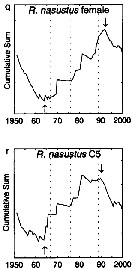 issued from : G.A. Rebstock in Global change Biology, 2002, 8. [p.77, Fig.2 q, r]. issued from : G.A. Rebstock in Global change Biology, 2002, 8. [p.77, Fig.2 q, r].
Climatic regime shifts and decadal-scale variability in calanoid copepod populations off southern California (31°-35°N, 117°-122°W.
Cumulative sums of nonseasonal anomalies from the long-term means of copepod abundance from years 1950 to 2000.
A negative slope indicates a period of below-average anomalies; a positive slope indicates a period of above-average anomalies. Abrupt changes in slope indicate step changes. Step changes are marked with arrows (upward-pointing for increases, downward -pointing for decreases).
The October 1966 cruise (prior to the increase in sampling depth), March 1976 cruise (prior to the 1976-77 climatic regime shift), and October 1988 cruise (prior to the hypothesized 1989 climatic regime shift) are marked with vertical lines. |
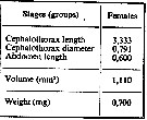 issued from : A.A. Shmeleva in Bull. Inst. Oceanogr., Monaco, 1965, 65 (n°1351). [Table 6: 5 ]. Rhincalanus nasutus (from South Adriatic). issued from : A.A. Shmeleva in Bull. Inst. Oceanogr., Monaco, 1965, 65 (n°1351). [Table 6: 5 ]. Rhincalanus nasutus (from South Adriatic).
Dimensions, volume and Weight wet. Means for 50-60 specimens. Volume and weight calculated by geometrical method. Assumed that the specific gravity of the Copepod body is equal to 1, then the volume will correspond to the weight.
In that case, the relation of the calculated weight appeared to be 1.5-2.4 more than the weight determined by weighting according to the method recommended by E.V. Borutsky (1934) and F.D. Mordukhy-Boltovsky (1954). |
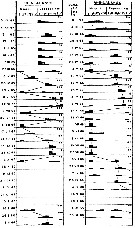 issued from : M.M. Mullin & E.R. Brooks in Limnol. Oceanogr., 1967, 12. [p.660, Fig.2]. issued from : M.M. Mullin & E.R. Brooks in Limnol. Oceanogr., 1967, 12. [p.660, Fig.2].
Relative abundance of the developmental stages of Rhincalanus nasutus at various times over a 2-yr period in the California Current, a few kilometers offshore from Scripps Institution of Oceanography (La Jolla, San Diego)
The number associated which each histogram shows the total number of individuals of all stages of that species caught with net in a 90-m vertical tow.
The height of the shaded bar associated with each developmental stage shows the relative contribution of that stage to this total. If less than 10 individuals were found in the samples from any date, no histogram was drawn. Before 23 March 1965, no nauplii were sampled, so frequencies are based on copepodite stages only. Diagonal lines connect supposed generations.
Nota : After Mullin & Brooks, the local field population apparently completed 4 successive generations in the 29 weeks between 23 March and 12 October 1965, averaging 7.25 weeks per generation.
The results for 1966 were less clear, especially during spring. One generation was apparently completed in about 7.5 weeks between 26 April and 17 June, but there was a long delay in the early naupliar stages of the next generation so that a third generation was not produced until October.
Hence, only 2 generations seem to have been produced in 1966 in the same period in which 4 generations had apparently been produced in 1965.
In laboratory cultures of R. nasutus in which eggs were produced, the eggs were laid 2 or 3 weeks after the appearanfe of adult females. This and the rate of development (shown in Table 1) give a minimum egg-to-egg generation time of 7 to 8 weeks, similar to that of the field popyulation during summer 1965.
Egg production in cultures continued for an average of 7 weeks, so that the time from an egg to the completion of egg production by the resulting female was about 15 weeks, although the life span of these females might be almost twice this.
Concerning the fecundity, Mullin & Brooks indicate under ideal conditions, the total number of eggs produced by wild females believed to have copulated only a short time before capture (many were still carrying spermatophores). Four groups involving 57 females, gave average values of 103, 214, and 355 viable eggs/female for 10 weeks of egg production. |
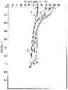 issued from : M.M. Mullin & E.R. Brooks in Limnol. Oceanogr., 1967, 12. [p.658, Fig.1]. issued from : M.M. Mullin & E.R. Brooks in Limnol. Oceanogr., 1967, 12. [p.658, Fig.1].
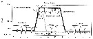
Vertical distribution of temperature at the sampling station in the California Current, a few kilometers offshore from Scripps Institution of Oceanography (La Jolla, San Diego) in various months (indicated by roman numerals). |
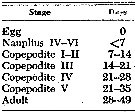 issued from : M.M. Mullin & E.R. Brooks in Limnol. Oceanogr., 1967, 12. [p.659, Table 1]. issued from : M.M. Mullin & E.R. Brooks in Limnol. Oceanogr., 1967, 12. [p.659, Table 1].
Approximate cumulative time (in days) required for development at 12°C in the laboratory based on 13 stocks of Rhincalanus nasutus. |
 Issued from : S. Shimode, K. Takahashi, Y. Shimizu, T. Nonomura & A. Tsuda in Deep-Sea Res. I, 2012, 65. [p.143, Fig.10, a]. Issued from : S. Shimode, K. Takahashi, Y. Shimizu, T. Nonomura & A. Tsuda in Deep-Sea Res. I, 2012, 65. [p.143, Fig.10, a].
Schematic illustration of the most probable life cycle of Rhincalanus nasutus (a). Ontogenetic vertical migration during the year in the Kuroshio-Oyashio transition area
C = copepodite stage; AF = female adult; AM = male adult.
Compare with Rhincalanus rostrifrons restricted to more southerly latitudes (15-37°N) in the NW Pacific.
Nota: Dormancy in deep waters (500-1000 m) by R. nasutus might indicate a strategy to avoid the relatively high predation risks incurred in shallower waters, due to its larger body size. In contrast, the smaller body size of R. rostrifrons facilitates dormancy in shallower waters (200-500 m depth). |
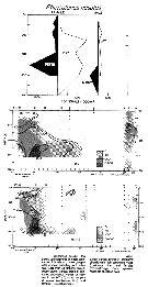
 Issued from : P.-E. Lapernat in DEA Océanogr. Biol., Univ. P. & M. Curie, Paris VI. July 5, 2000. [Fig.9 b]. Issued from : P.-E. Lapernat in DEA Océanogr. Biol., Univ. P. & M. Curie, Paris VI. July 5, 2000. [Fig.9 b].
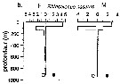
Verical distribution of Rhincalanus nasutus at an eutrophic site (off Mauritanian coast: 20°32 'N, 18°36' W) in females (F) and males (M) (ind. per m3) in the day (white circle) and night (black circle).
Nota: Sampling in the water column 0-1000 m, one during the day and another during the night with BIONESS multiple-net: 0-75; 75-150; 150-250; 250-350; 350-450; 450-550; 550-700; 700-850; 850-965 m. In May-June 1992. |
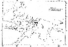 Issued from : A. Fleminger inComposite stations of the Siboga Expedition (1899), the Snellius Expedition (1929) and R/V ''Alpha Helix'' Moro Expedition (1979). Issued from : A. Fleminger inComposite stations of the Siboga Expedition (1899), the Snellius Expedition (1929) and R/V ''Alpha Helix'' Moro Expedition (1979).
Stations are indicated by small filled circles, Calanoides philippinensis records by open diamonds, and Rhincalanus nasutus records by a large filled circles.Note how positive records are concentrated off southwestern New Guinea. |
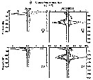 Issued from : M.D. Ohman, A.V. Drits, M.E. Clarke & S. Plourde in Deep-Sea Res. II, , 1998 , 45. [p.1719, Fig. 4 B]. Issued from : M.D. Ohman, A.V. Drits, M.E. Clarke & S. Plourde in Deep-Sea Res. II, , 1998 , 45. [p.1719, Fig. 4 B].
Vertical distribution of copepod in the San Diego Trough in June and December. Adult female and copepodid stage V of Rhincalanus nasutus.
Dark symbols illustrate nightime distributions, open symbols illustrate daytime distributions, each plotted at the mid-point of the sampling interval. Sampling extended deeper in December than in June.
Sampling out in the San Diego Trough (near 32°50'N, 117°40'W) in 6-14 June 1992 and 15-22 December 1992.
For the authors, the species appears to enter dormancy as adult females, although the evidence is equivocal. |
 Issued from : M.D. Ohman, A.V. Drits, M.E. Clarke & S. Plourde in Deep-Sea Res. II, , 1998 , 45. [p.1730, Table 3]. Issued from : M.D. Ohman, A.V. Drits, M.E. Clarke & S. Plourde in Deep-Sea Res. II, , 1998 , 45. [p.1730, Table 3].
Differential dormancy of co-occuring copepods in the California Current System in the San Diego Trough.
Indices used to differentiate actively growing from dormant animals included developmental stage structure and vertical distribution; activity of aerobic metabolic enzymes (Citrate Synthase and Electron Transfer System complex); investment in depot lipids (wax esters and triacylglycerols); in situ grazing activity from gut fluorescence, and egg production rates. |
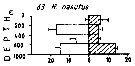 Issued from : M. Madhupratap & P. Haridas in J. Plankton Res., 12 (2). [p.313, Fig.6]. Issued from : M. Madhupratap & P. Haridas in J. Plankton Res., 12 (2). [p.313, Fig.6].
Vertical distribution of calanoid copepod (mean +1 SE), abundance No/100 m3. 63- Rhincalanus nasutus.
Night: shaded, day: unshaded.
Samples collected from 6 stations located off Cochin (India), SE Arabian Sea, November 1983, with a Multiple Closing Plankton Net (mesh aperture 300 µm), in vertical hauls at 4 depth intervalls (0-200, 200-400, 400-600, 600-1000 m). |
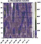
 Issued from : Y.-Q. Chen in CalCOFI Rep., 1986, XXVII. [Fig.6, p.214]. Issued from : Y.-Q. Chen in CalCOFI Rep., 1986, XXVII. [Fig.6, p.214].
Vertical abundance of females, males and late copepodites.
Nota: The distribution during the Krill Expedition in the Pacific east tropical (23°N to 3°S) is restricted to the middle and maximum depths sampled. South of 8°N its distribution appears to have influenced by the Equatorial Counter-current. The maximum concentration occurred between 500 and 600 m. At station 21, the maximum number of females was 11,000 individuals/m3 about 500 m. From 20°N to near the equator, this species was not present from middle depths to the surface. Numbers of females were higher than those of the male, and diel vertical migration was not apparent.
The mean percentage combined was 9.6% (day: 5.9, night: 13.2) for all samples with the bongo net .
See in Subeucalanus subtenuis figs.1, 12, 13). |
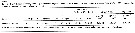 Issued from : M. Bode, R. Koppelmann, L. Teuber, W. Hagen & H. Auel inGlobal Biogeochemical Cycles, 2018, 32. [p.844, Table 1). Issued from : M. Bode, R. Koppelmann, L. Teuber, W. Hagen & H. Auel inGlobal Biogeochemical Cycles, 2018, 32. [p.844, Table 1).
Cf. explanations of these measures in Calanoides natalis from the same authors.
Compare with Rhincalanus cornutus. |
 Issued from : M. Bode, A. Schukat, W. Hagen & H. Auel in J. Exp. Mar. Biol. Ecol., 2013, 444. [p.3, Table 1]. Issued from : M. Bode, A. Schukat, W. Hagen & H. Auel in J. Exp. Mar. Biol. Ecol., 2013, 444. [p.3, Table 1].
Dry mass, individual respiration rate and ETS activity from the northern Benguela Current upwelling system along transects at 23°S and 26°40'S, off Walvisbay and Lüderitz (Namibia).
Relationship between individual ETS activities and individual respiration rates; mean ETS activities with standard deviations are plotted again mean respiration rates (Cf. in Calanoides natalis. The letters besides each point identifies the associated species in Table 1 (e, g, for this species) in the same authors.
Cf. Table 1: Dry mass, individual respiration rate and ETS activity.
For Conover & Corner (1968) the female respiration rate at 3-5°C were 0.39 µl O2 h ind-1 (DM: 529 µg) in the North Atlantic; For Conover (1960) at 7°C: 0.59-0.65 (DM: 826-1079 µg) North West Atlantic. |
 Issued from : M. Bode, A. Kreiner, A.K. van der Plas, D.C. Louw, R. Horaeb, H. Auel & W. Hagen in PLoS ONE, 2014, 9 (5). [p.9, Fig.9, e]. Issued from : M. Bode, A. Kreiner, A.K. van der Plas, D.C. Louw, R. Horaeb, H. Auel & W. Hagen in PLoS ONE, 2014, 9 (5). [p.9, Fig.9, e].
Monthly abundances (no. m-2 along transect from inshore (0 nm) to offshore (70 nm) (See map).
Note patches in the spatial distributions from inshore (0 nm) and offshore (70 nm).
Compare with Calanoides natalis, Metridia lucens, Nannocalanus minor from the same authors. |
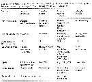
| | | | Loc: | | | Antarct. (SW Atlant., SE Pacif.), South Georgia, Magallones region, sub-Antarct. (SW Atlant., Indian, SW & SE Pacif.), South Africa (E & W, STC region), Saldanha Bay, Namibia, Angola, Baia Farta, Dakar, off Mauritania-NW Cape Verde Is., Morocco-Mauritania, Cap Ghir, Canary Is., off Madeira, Portugal, off W Cabo Finisterre, Bay of Biscay, Argentina (southern offshore), Uruguay (continental shelf), Cabo Frio, off Rio de Janeiro, S Brazil, Argentina, Barbados Is., Yucatan, G. of Mexico, Caribbean, off Bermuda, Sargasso Sea, Station "S" (32°10'N, 64°30'W), off Cape Hatteras, off E Cape Cod, Delaware Bay (outside), Chesapeake Bay, Long Island, G. of Maine, off Woods Hole, Bay of Fundy, off SE Nova Scotia, S Davis Strait, Strait of Denmark, Fram Strait, Kongsfjorden, Spitzbergen, Wyville Thomson Ridge, Iceland, Faroe Is., Arct. (Nansen Basin), Barents Sea, Norway, Raunefjorden (rare), W & SW Ireland, North Sea, Ibero-moroccan Bay, Gibraltar Strait, Medit. (M'Diq, Alboran Sea, Habibas Is., Sidi Fredj coast, Algiers, Banyuls, Marseille, Ligurian Sea, Tyrrhenian Sea, G. of Gabes, Adriatic Sea, Black Sea), G. of Aqaba, off Sharm El-Sheikh, G. of Eilat, Red Sea, G. of Aden, G. of Oman, Arabian Sea, Somalia, Maldive Is., off Cochin, Natal, India (Saurahtra coast, Lawson's Bay, Porto Novo, Gulf of Mannar), N Indian, off S Madagascar, Nosy Bé, S Indian (subtropical convergence), E India, Bay of Bengal, Indonesia-Malaysia, Lombok Sea, Flores Sea, Arafura Sea, Banda Sea), Philippines, Viet-Nam (Cauda Bay), G. of Tonkin, China Seas (East China Sea, South China Sea), Taiwan, Kuroshio Current, S Korea S, Tsushima Straits, Japan, Kuchinoerabu Is., Kuroshio-Oyashio transition, off NE Japan, off S Shikoku Is., Station Knot, off SE Japan, Arct. (Nansen Basin), Aleutiian Is., British Columbia, Bay of Seattle, off Washington coast, Oregon (Yaquina, off Newport), California, Santa Monica Basin, W Baja California, Bahia Magdalena (rare), Gulf of California, La Paz, Guaymas Basin, W Mexico, G. of Tehuantepec, W Costa Rica, Pacif. (E equatorial), Australia (Great Barrier, New South Wales), New Zealand (Kaikoura), New Caledonia, off W Guatemala, Pacif. (equatorial & subtropical), off Panama, Bahia Cupica (Colombia), off Galapagos, off Peru, Pacif. (SE tropical), Chile ( N-S, off Valparaiso, off Santiago, Concepcion), Straits of Magellan | | | | N: | 386 | | | | Lg.: | | | (7) F: 5-4,5; M: 4,5-3,8; (14) F: 4,7-4,5; (22) F: 5,1-3,9; M: 3,8-2,7; (28) F: 4,75-3,85; M: 3,55; (35) F: 5-4,5; (36) F: 6,08-5,63; (38) F: 4,8-4,15; (45) F: 5,5-4; M: 4-3; (47) F: 5,1-3,9; M: 3,8; (54) F: 2,85; M: 4,3; (75) F: 4,94-2,82; (101) F: 4,37-4,08; (104) F: 4,7; M: 3,5; (116) F: 5,18; (125) F: 4,5-3,6; M: 3,81-3,74; (131) F: 6,1-3,7; (135) F: 3; M: 2,7; (142) F: 3; M: 2,7; (199) F: 5,6-4,26; M: 4,33-3,57; (207) F: 4,28-4,2; M: 3,51; (208) F: 4,8-3,9; (237) F: 4,5; (254) F: 4,7; (327) F: 5,81-4,31; M: 3,93; (290) F: 3-4,25; M: 3,35-3,4; (340) F: 3,8; (432) F: 5,2-4,2; (530) F: 4,2; M: 4; (785) F: 3,49-3,26; (786) F: 4,52-3,6; M: 3,67-3,45; (991) F: 3,9-5,5; M: 2,7-4; (1122) F: 4,05; M: 3,35; {F: 2,82-6,10; M: 2,70-4,50}
Chiba S. & al., 2015 (p.971, Table 1: Total length female (June-July) = 3.3 mm [optimal SST (°C) = 9.6].
For Hidalgo & al. (2012) copepodids V lengths: Prosome female: 3.5; urosome female: 0.6; prosome male: 3.7; urosome male: 0.7. | | | | Rem.: | épi à bathypélagique.
Sampling depth (Antarct., sub-Antarct.) : 0-500-4000 m. 280-450 m (Pipe & Coombs, 1980 at 60°N, 07°W).
Voir aussi les remarques en anglais | | | Dernière mise à jour : 28/10/2022 | |
|
|
 Toute utilisation de ce site pour une publication sera mentionnée avec la référence suivante : Toute utilisation de ce site pour une publication sera mentionnée avec la référence suivante :
Razouls C., Desreumaux N., Kouwenberg J. et de Bovée F., 2005-2026. - Biodiversité des Copépodes planctoniques marins (morphologie, répartition géographique et données biologiques). Sorbonne Université, CNRS. Disponible sur http://copepodes.obs-banyuls.fr [Accédé le 10 février 2026] © copyright 2005-2026 Sorbonne Université, CNRS
|
|
|
|


;)
;)
;)
;)
;)
;)
;)
;)
;)
;)
;)
;)
;)
;)
;)
;)
;)
;)
;)
;)
;)
;)
;)
;)
;)
;)
;)
;)
;)
;)
;)
;)
;)

;)
;)
;)
;)
;)
;)
;)
;)
;)
;)
;)