An Overview and Initial Interpretation on the Diversity and Geographic Distribution of Pelagic Copepoda

---

Interactive distribution map

The different oceanic zones : Summary of the species - Marine currents and other maps

The following tables summarise for the various oceanic zones concerned: the total number of species (named forms only) and their percentage with respect to all copepod species, and the percentage with respect to the total number of species in the zone (ind.: indicates forms without a denomination cited as sp. by authors).

Zones: Indian Ocean (16) ; Red Sea (15)

	16	15
Total species:	963 (37.5 %) (+ 30 ind.)	280 (10.9 %) (0 ind.)
Calanoida:	773	156
other orders	190	124

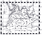Issued from : T.S.S. Rao in Zoogeography of the Indian Ocean. Edis.: S. Van der Spoel & A.C. Pierrot-Bults, 1979. [p.255, Fig.1]
Surface currents in the Indian Ocean. 1 = SW monsoon, 2 = NE monsoon, 3 = Hydrothermal Front, 4 = Upwelling.

Sewell (1948, p.435) recorded 270 known species in the Indian Ocean. Of the 56 endemic species he reported (Sewell 1948, p.429), 26 have never been reported in any other ocean and 15 are known from a geographical extension encroaching upon neighbouring geographical zones . 486 species are also found in the Indo-Malay archipelago, i.e. 48.9 %

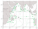A schematic representation of identified current branches during the Southwest Monsoon, including some choke point transport numbers (Sv=10⁶m³s^-1). Current branches indicated are the South Equatorial Current (SEC), South Equatorial Countercurrent (SECC), Northeast and Southeast Madagascar Current (NEMC and SEMC), East African Coast Current (EACC), Somali Current (SC), Southern Gyre (SG) and Great Whirl (GW) and associated upwelling wedges, Socotra Eddy (SE), Ras al Hadd Jet (RHJ) and upwelling wedges off Oman, West Indian Coast Current (WICC), Laccadive High and Low (LH and LL), East Indian Coast Current (EICC), Southwest and Northeast Monsoon Current (SMC and NMC), South Java Current (JC) and Leeuwin Current (LC).
Issued from : F.A. Schott & J.P. McCreary Jr. in Progress in Oceanography: An Annual Review, 2001, 51. [p.13, Fig.8].

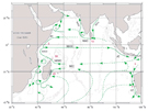A schematic representation of identified current branches during the Northeast Monsoon, including some choke point transport numbers (Sv=10⁶m³s^-1). See figure above for acronyms.
Issued from : F.A. Schott & J.P. McCreary Jr. in Progress in Oceanography: An Annual Review, 2001, 51. [p.14, Fig.9].

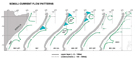Schematic diagram of the Somali Current upper-layer flow patterns over the course of the year. Also marked are undercurrents as presently known (after Schott et al., 1990, with revisions). See figure above for acronyms.
Issued from : F.A. Schott & J.P. McCreary Jr. in Progress in Oceanography: An Annual Review, 2001, 51. [p.39, Fig.32].

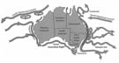Major currents and circulation patterns around Australia.
The continent is bounded by the pacific ocean to the east, the indian Ocean to the west and the Southern Ocean to the south.
Issued from : E.S. Poloczanska & al. in Oceanography and Marine Biology: An Annual Review, 2007, 45. [p.409, Fig.2]. Figure courtesy of S. Condie/CSIRO.

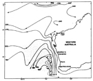Representation of the major features of the circulation of the southeastern Indian Ocean.
Geopotential anomaly contours (full line) after Wyrtki (1961), (dotted) after Andrews (1975, 1977), and the Leeuwin Current modified from Cresswell & Golding (1980, dashed) are surimposed on the known extent of the larval distribution of Panulirus cygnus shown as a shaded area.
Issued from : B.F. Phillips in Oceanogr. Mar. Biol. Ann. Rev., 1981, 19. [p.31, Fig.21].

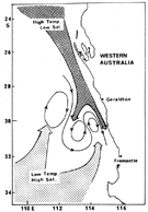Idealized representation of the two major water types found in the southeastern Indian Ocean (after Kitani, 1977).
B.F. Phillips in Oceanogr. Mar. Biol. Ann. Rev., 1981, 19. [p.30, Fig.20].

Indian Ocean currents:

Equatorial Current:
South of the equator, around 10° South latitude, the general movement of the waters traces a vast cyclonic circuit, quite comparable to that of the other oceans.
The South Equatorial Current flows from East to West, parallel to the equator. This current, with a speed of 20 to 25 miles per day, never crosses the equator. Its northern limit, which varies like that of the Southeast trade winds, generally lies between 4° and 10° South. Its southern limit extends in places as far as the 25th parallel (the parallel of southern Madagascar). The enormous mass of water it carries westward is obstructed by Madagascar. It begins to split near the islands of Réunion and Mauritius: one branch passes north of Madagascar, the other south.

Mozambique Current:
The northern branch of the Equatorial Current, which rounds Cape Amber (Madagascar) at a westward speed of 1 to 3 knots, reaches the African coast at the latitude of Cape Delgado, situated approximately on the parallel of Cape Amber. Part of it bends southwestward and becomes the Mozambique Current, which runs along the African coast, its flow and speed varying with the season. The current is much more regular and stronger during the Northern Hemisphere's Northeast monsoon (from November to January its speed reaches 1 knot, whereas it is only half a knot from May to July).

Agulhas Current:
The southern branch of the Equatorial Current passes south of Madagascar at a speed of half a knot and joins the Mozambique Current off Natal. Their confluence forms the Agulhas Current, which is felt as far as 120 miles from land and carries relatively warm waters as far as the Cape of Good Hope.
The Agulhas Current, one of the most powerful of the ocean currents, is also one of the most constant. Along the Natal coast its speed reaches 4 knots, sometimes 5, and is rarely below 2 knots.
The Agulhas Current does not appear to show a regular annual variation in volume, strength or direction. It may be somewhat weaker in July, when the Southwest monsoon blows in the northern Indian Ocean and the Mozambique Current, which partly feeds it, is weaker.
Westerly gales, fairly frequent at these latitudes, sometimes oppose it, but it then becomes more violent, as though the temporary barrier raised by the wind had built up its waters, which are subsequently released. This creates a dangerous sea, especially on the southeastern edge of the Agulhas Bank. Over the bank itself, at depths of less than 120 metres, the sea is much calmer. The current tends to follow the contours of the bank without crossing over it toward land. A small portion passes over the southern tip of the bank, or skirts around it, to rejoin, beyond the Cape of Good Hope, the current running along the west coast of southern Africa, which flows northward. Warm waters rarely reach Table Bay (Cape Town), where the water is much colder than in Simon's Bay.
The main body of the Agulhas Current flows southward as far as the parallel of 40° South, where it bends eastward to join the Southern Ocean Current, which comes from the Southwest and West-Southwest.
The meeting of the warm, saline waters of the Agulhas Current with the cold, less saline waters of the Southern Ocean Current creates, between the parallels of 37° and 40° South, a region of variable currents and turbulence, where temperature and salinity change rapidly from one point to another: temperature differences of 10°C have been recorded between points close together. The line where the currents meet is marked by a change in the colour of the water.

Coastal countercurrents:
The Mozambique Current and, above all, the Agulhas Current are only clearly directed southwestward at a distance of at least 3 miles from land. Closer to shore, countercurrents occur, flowing toward the Northeast and East, and at times toward land, where tidal currents are significant. In the vicinity of Cape Agulhas there is a countercurrent flowing northward (i.e. toward land) at a speed sometimes exceeding 1 knot.

Southern Indian Ocean Current:
Formed by the meeting of the warm Agulhas Current with the colder current coming from the West-Southwest, it flows Eastward and East-Northeastward; its average speed is about 1.5 knots, though higher speeds, reaching 3 knots, have been recorded.
The current is stronger and lies further north in summer than in winter; it can be found as far south as latitude 50°. Further East, its speed decreases; near the Kerguelen Islands it is no more than a fairly slow drift, of about ten miles per day, which merges, south of Australia, with the drift of the southern Pacific Ocean.

Currents off Southwest Australia:
Along the west coast of Australia, between Cape Leeuwin and Point Cloates, the current generally flows Northwestward, at a speed of 1 to 1.5 knots. This current is strongly affected by the wind. During winter, near the coast, it is replaced by a southward-flowing current.

Sub-equatorial and northern currents:
In the northern part of the Indian Ocean, the currents show a remarkable seasonal variation. The movement of the waters broadly follows that of the air masses, governed by the Northeast monsoon during the boreal winter and the Southwest monsoon during the boreal summer.
During the Northern Hemisphere winter, at the time of the Northeast monsoon, the currents flow Westward, both in the Arabian Sea and in the Bay of Bengal. Sri Lanka is entirely washed, to the North and South, by the waters of this current.
In the Bay of Bengal, at the latitude of Madras, the current bends Northward and describes a clockwise circuit. At the outlet of the Strait of Malacca, the current has a speed of 2 to 3 knots.
In the Arabian Sea, the speed of the Westward and Southwestward current does not reach 1 knot; it exceeds 2 knots in the Gulf of Aden, especially off the Arabian coast (off the Somali coast, an eastward-flowing countercurrent of about 1 knot is often observed). As it bends Southward along the Somali coast, the current gains further speed (J. Rouch measured 84 miles per day on a crossing from Guardafui (Ras Asir) to Zanzibar).

Equatorial countercurrent:
Between these westward-flowing currents and the South Equatorial Current, an eastward-flowing equatorial countercurrent is observed, whose northern limit is the equator and whose southern limit lies at about the 6th parallel. The speed of this countercurrent is highly variable: fairly weak at its point of origin near the African coast (1 to 1.5 knots), while toward the middle of the Indian Ocean, where the countercurrent passes between the Maldives and the Chagos Archipelago, its speed can reach 3 knots.

During the Northern Hemisphere summer, the Southwest monsoon is the prevailing wind in the northern Indian Ocean. The currents change direction along with the winds. Under these conditions, instead of flowing Westward and Southwestward, they flow Eastward and Northeastward.
The highest speeds of the summer monsoon current are found along the Somali coast and around Sri Lanka. Along the Somali coast, the highest speed recorded was 133 miles per day (over 5 knots). This high current speed results from the strength of the Southwest monsoon, which reaches 12, and even 15, metres per second.
150 miles south of Socotra, the current is deflected by the shallow depths (between Socotra Island and Ras Asir). On the parallel of Ras Hafun, the current flows Eastward as far as the meridian of Socotra, then Southeastward, maintaining a speed of 4 knots. A current of 7 knots, flowing East-Southeast, has even been recorded 170 miles south of Socotra. Since in these waters the Southwest monsoon is neither deflected nor weakened, where the monsoon meets the Southeastward current there is a zone where the sea is particularly rough (between 8° and 11° North latitude and 53° and 58° East longitude).
Near Sri Lanka, the current speed does not appear to exceed 3.5 knots.
In the Gulf of Aden, a westward-flowing countercurrent is observed along the African coast, so that on this coast, in all seasons, the current always runs opposite to the wind blowing over the Gulf of Oman.

Current changes are not simultaneous with monsoon changes. On the whole, the Northeastward and Eastward currents last longer than the Westward and Southwestward currents.

The eastern coast of Sri Lanka and the Indian peninsula are linked by a chain of islands and coral reefs forming Adam's Bridge; this topography allows the seasonal changes of the current to be observed with precision. Between one of these islands, Rameswaram Island, and the Indian coast, there is a channel 3 to 4 metres deep and 25 to 60 metres wide, where the current reverses direction with the monsoon: Southward with the Northeast monsoon, Northward with the Southwest monsoon. When the monsoon is well established, the speed of this current reaches 7 knots.

The Arabian Gulf:
In the Arabian Gulf, where the tidal range is relatively large and depths are shallow, tidal currents dominate; their speed reaches 3 knots at several points. In summer, the Southwest monsoon drives the waters into the Gulf; in winter, during the Northeast monsoon, the opposite movement occurs.

References:
J. Rouch, Traité d'Océanographie physique. Les mouvements de la mer. Vol. 3. Édit. Payot, Paris, 1948.
National Geographic Society, Washington D.C., 1981, pp.228-229
Atlas of Pilot Charts http://msi.nga.mil/NGAPortal/MSI.portal?_nfpb=true&_pageLabel=msi_portal_page_62&pubCode=0003 NATIONAL GEOSPATIAL-INTELLIGENCE AGENCY (USA)

The Red Sea contained 111 species of which the majority are originally from the Indo-Pacific region (Sewell, 1948, p.435). With 280 species this number is still one of the lowest, due in part to the restricted opening into the Indian Ocean, but probably also to the limited number of sampling cruises. Analysis shows that 229 species are shared with the Indian Ocean, and 217 with the Mediterranean. 239 of these relatively cosmopolitan species are also found in several other zones.

Red Sea currents:
Disregarding tidal currents, which are mainly felt at the northern and southern ends of the Red Sea, namely in the Gulf of Suez and the Strait of Bab-el-Mandeb, the currents depend on the monsoons of the Indian Ocean.
From October to March (the period of the Northeast monsoon) the current flows North-Northwestward in the Strait of Bab-el-Mandeb, where it reaches a speed of 1 to 2 knots, and this current can sometimes be felt as far as the northern Red Sea.
From June to September (the period of the Southwest monsoon) the current flows South-Southeastward from the middle of the Red Sea to the Strait of Bab-el-Mandeb, where its speed is 30 to 40 miles per day. In the northern Red Sea, a North-Northwestward current is often still observed during this season.
References:
J. Rouch, Traité d'Océanographie physique. Les mouvements de la mer. Vol. 3. Édit. Payot, Paris, 1948.
National Geographic Society, Washington D.C., 1981, pp.228-229
Atlas of Pilot Charts http://msi.nga.mil/NGAPortal/MSI.portal?_nfpb=true&_pageLabel=msi_portal_page_62&pubCode=0003 NATIONAL GEOSPATIAL-INTELLIGENCE AGENCY (USA)

 

Zones: G. of Thailand, Indo-Malay Archipelago (17) ; China Seas (21)

	17	21
Total species:	649 (25.3 %) (+ 8 ind.)	643 (25 %) (+ 6 ind.)
Calanoida:	531	492
other orders	118	151

Copepoda have not been intensively studied in the Indo-Malay Archipelago since the work of A. Scott (1909) who recorded 326 species (not including Lichomolgidae). Vervoort (1946) et Wilson (1950) contributed to knowledge of the fauna of this region. In view of the large number of islands of all sizes and the deeps that separate them, the total number of species in this zone has probably been vastly underestimated. 380 species, i.e. 57.8 %, are shared with tropical and subtropical zones in the Pacific.

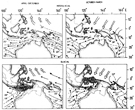Issued from : A. Fleminger in UNESCO Techn. papers mar. Sci., 1986, 49. [p.89, Fig.5].
Sea surface temperature isotherms, °C, surface currents (slender arrows) and Northeast Trade Winds (thick arrows) in eastern Indo-Australian region.
Top two panels show conditions in southern hemisphere winter and summer conditions in the present time and hypothetized for past interglacial stages.
Bottom two panels show conditions thought to prevail during Pleistocene glacial stages. Oblique line shading show areas in which unusually cool (<21°C) surface temperatures may have predominated seasonally and acted as a barrier to the passage of mixed layer stenotherms; land area extended to 200 m isobath to approximately lowered eustatic sea level during glacial stages (modified from Webster & Streten, 1972; Brinton, 1975).

Nota : Dotted shading in the area of Wallacea represents special local conditions that would have lowered surface temperatures on a seasonal basis. Quinn (1971) argues for increased upwelling in equatorial latitudes of the westernmost Pacific during Pleistocene glacial stages. He notes the existence of fossil guano deposits on equatorial islands lying west of the Gilberts Islands, which indicates the past presence of large colonies of sea birds on islands now lacking such colonies.
Presumably during Pleistocene glacial periods, equatorial upwelling in the west Pacific provided the ressources to support the now extinct bird colonies. In general over the past 75000 years, fluctuations in the intensity of the trade winds has been concurrent or preceded fluctuations in the amount of ice stored on continents and wind velocityn of the winter trades intensified during cool climatic stages of the earth and diminished during warm stages (Molina-Cruz, 1977).
Pleistocene glacial stages appear to have persisted for periods of tens of thousands of years.
Bé & Duplessy (1976) indicates that the glacial stages persisted for tens of thousands of years several times during the million years of the Pleistocene. For stenothermal species ranging years (1976) show that the half-million-year records for the western Indian Ocean and the quarter-million-year record for te eastern Indian Ocean had cold conditions prevailing for more than half of their respective periods. Van Andel & al. (1967) and Webster & Streten (1972) believe that cool water entered the Timor Sea during Pleistocene glacial stages based on an intensification of the cool, west Australian boundary current an dits more northward penetration. Changes in current intensity during Pleistocene glacial stages have been recorded off South Africa (Hutson, 1980).
In the northern hemisphere during Pleistocene glacial winters, the NE Trades probably intensified sufficiently to induce coastal upwelling off northwest New Guinea and the eastern Moluccas. Webster & Streten (1972) suggest that surface temperatures off northwest New Guinea ranged from 22 to 24°C, while the CLIMAP Project (1976) indicates 25 to 27°C in the southern hemisphere winter for this area. Reducing these values by 3°C, the extent surface temperatures are lowered in upwelling plumes off New Guinea, would depress winter Pleistocene surface temperatures to a range of 19 to 24°C, i .e., well below present-day winter conditions. Assuming that the median, 21.5°C, is close to actual surface temperatures in upwelling plumes of the Pleistocene glacial winter, the northern end of Wallacea would be inhospitable to tropical stenotherms roughly from October to March. In the southern hemisphere's winter, the West Australia Boundary Current would intensify and the SE Trades might cause coastal upwelling along the Sehul shelf. It is reasonable to expect winter surface temperatures of about 20°C in the Timor and Banda Seas (as shown by Webster & Srreten, 1972), rendering the southern end of Wallacea inhospitable to surface-bound stenotherms roughly between April and September.
The hypothetized glacial-stage conditions shown in the lower two panels of figure 5 would enhance C. philippinensis and Rhincalanus nasutus population expansions, while depressing populations of sternothermal pontellids.
Stratigraphic evidence by Bé & Duplessy (1976) indicates that the glacial stages persisted for tens of thousands of years several times during the million years of the Pleistocene. For stenothermal species ranging across Wallacea, each glacial sequence would interrupt their distribution and provide an opportunity for the allopartic subpopulations to diverge.
If Wallacea was a long-term barrier to passage of stenothermal species of the mixed layer, we should expert to see evidence of its vicariant role in speciation patterns of locally distributed species groups. That is, sister species may be expected to have allopatric or parpatric distributions extending from Wallacea.

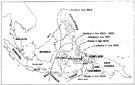Biogeographic bounderies proposed for separating the Oriental and the Australia/New Guinea faunal regions (see George, 1981).
Issued from : A. Fleminger in UNESCO techn. Pap.Mar. Sci., 1986, 49. [p.84, Fig.1].

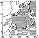Topographic feature of the Kuroshio region (modified from Mogi, 1972).
Ridges: A, Izu-Ogasawara; B, Mariana; C, Yap; D, Kyushu-Palau; E, Daito, F, Ryukyu.
Basins: 1, Shikoku; 2, West Mariana; 3, Philippines; 4, South China Sea.
Others: I, Okinawa Trough; II Bashi Channel; III, Sakishima Depression; IV, Tokara Strait.
Issued from : J.L Su, B.X. Guan & J.Z. Jiang in Ann. Rev., 1990, 28. [p.13, Fig.2].

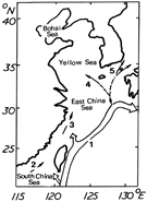Schematic picture of the Kuroshio Current and its branches in the China Seas: 1, Kuroshio Current; 2, South China Sea Warm Current; 3, Taiwan Warm Current; 4, Yellow Sea Warm Current; 5, Tsushima Current.
Issued from : J.L Su, B.X. Guan & J.Z. Jiang in Ann. Rev., 1990, 28. [p.37, Fig.22].

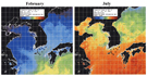Issued from : M.-C. Jang, S.H. Baek, P.-G. Jang, W.-J. Lee & K. Shin in Ocean and Polar Res., 2012, 34 (1). [p.40, Fig.2].
Weekly average sea surface temperature (SST) derived from NOAA/AVHRR during periods in February and July 2009 in the Korea Strait.
Sampling stations are marked as circles.

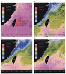Issued from : L.-C. Tseng, R. Kumar, H.-U. Dahms, Q.-C. Chen & J.-S. Hwanh in Zool. Studies, 2008, 47 (1). [p.53, Fig.4].
Monthly average sea-surface temperatures (SSTs) derived from averaged hourly recordings (AVHRRs) for (A) Aug. 1998, (B) Dec. 1998, (C) Mar. 1999, and (D) May 1999.

Nota: The Taiwan Strait is a relatively shallow (with an average depth of 60 m), 350 km long, and 180 km wide channel between the island of Taiwan and the southeastern Chinese coast, connecting the two marginal seas of the western Pacific, the East China Sea and the South China Sea.
In the Taiwan Strait there is a congruence of 3 different water masses (East China Sea, South China Sea), and the water masses representing the Kuroshio Current of the western North Pacific such hydrographic conditions affect the zooplankton community composition in the Taiwan Strait..
Wind patterns in this region are determined by the typical East Asian monsoon that is from the northeast (NE) during winter (Oct.-Mar.) and from southwest (SW) during summer (May-Aug.).
During the NE monsoon the China Coastal Current with low temperatures, low salinities, and high nutrient levels moves southwards driving zooplankton from the Bohai Sea, the Yellow Sea, and the East China Sea towards the Taiwan Strait.
Throughout the year, the warm, highly saline, and nutrient-poor Kuroshio Branch Current intrudes into the Taiwan Strait through the northern South China Sea and along the coast of southwestern Taiwan. However, during the prevailing NE monsoon period , the southherly flowing China Coastal Current near the Penghu Channel, south of the Changyun Ridge in the southeastern Taiwan Strait.
In spring when the NE monsoon weakens the Kuroshio Branch Current moves northward along the local isobaths into the northern part of the Taiwan Strait. Conversely, under the prevailing winds of the SW monsoon (May-Aug.), the South China Sea Warm Current with intermediate temperatures, salinities, and nutrient levels intrudes into the Taiwan Strait and moves northward together with the Kuroshio Branch Current that transports plankton from the northern South China Sea.
The hydrographic properties of this part (NW Taiwan) of the Taiwan Strait are mainly influenced by the NE and SW monsoons. The influence of cold water masses disappears during summer with increasing strength of the SW monsoon as water masses from the northern part of the South China Sea enter the Taiwan Strait and influence the hydrography around the west coast of Taiwan, and Guangdong and Fujian Provinces, China.

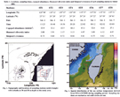Issued from : Y.-C. Lan, M.-A. Lee, C.-H. Liao & K.-T. Lee in J. Mar. Sci. Techn., 2009, 17 (1). [p.2, Table 1, Figs. 1, 2].
Copepod community structure of the winter frontal zone induced by the Kuroshio branch current and the China coastal current in the Taiwan Strait.

Nota: Copepods collected with a Bongo plankton net (mesh aperture: 335 µm), towed obliquely.
At each station, temperature and salinity at different depths were obtained by CTD profiler from the sea surface to a depth near the bottom. NOAA satellites provide SST measurements showing the spatial distribution of surface temperature with 1.1 km spatial resolution.

Chen, B (1986) records 345 species in the China Seas from the Bohai Sea and the Yellow Sea at 40° N to the eastern and southern tropical China Seas .

Zhang, W (2007) divides the China Seas into four sub-areas (South China Sea, East China Sea, Yellow Sea and Bohai Sea) ( See the interactive distribution map ). Concerning the division position of the sub-areas, in China, the line connecting Cheju Island and north bank of Yangtze River is the division line of Yellow Sea and East China Sea. The line connecting Nanao Island of Guangdong Province and Eluanbi of Taiwan Island is the division line of the East China Sea and South China Sea. About the ascription of sea east of Taiwan Island Zhang proposes that this area should be included into South China Sea due to the oceanic water properties.
The limits, however, are somewhat artificial, not taking into account movement of masses of water in time and space, and some species are so redundant with those of southern Japan (zone 22) and northern Malaysia and west of the Philippines (zone 17).

Currents in the China Seas:
The currents in the China Seas are mainly monsoon currents.
During the Northeast or North monsoon, from October to March, the currents flow toward the South and Southwest.
During the Southwest and South monsoon, from June to August, the currents flow toward the North and Northeast.
During the intermediate seasons, April-May on one hand, September to early October on the other, the currents are more irregular and variable.
The speed of these monsoon currents can exceed 1 knot, especially near the coasts. It reaches nearly 3 knots during the Southwest monsoon in the Taiwan Strait.
In the eastern part of the northern China Sea, between Taiwan and Japan, the Kuroshio passes through the Ryukyu Islands and is felt west of these islands. Its speed reaches 3 knots; its warm, dark blue waters are clearly distinct from the coastal waters, several degrees colder and yellowish-green in colour, which flow in the opposite direction during winter.
References:
J. Rouch, Traité d'Océanographie physique. Les mouvements de la mer. Vol. 3. Édit. Payot, Paris, 1948.
National Geographic Society, Washington D.C., 1981
Atlas of Pilot Charts http://msi.nga.mil/NGAPortal/MSI.portal?_nfpb=true&_pageLabel=msi_portal_page_62&pubCode=0003 NATIONAL GEOSPATIAL-INTELLIGENCE AGENCY (USA)

 

Zones: Japan (22) ; NW North Pacific (23)

	22	23
Total species:	711 (27.7 %) (+ 8 ind.)	369 (14.4 %) (+ 2 ind.)
Calanoida:	556	305
other orders	155	64

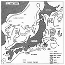Warm and cold currents around Japan and fishing grounds for pelagic fish, such as skipjack, tuna and squid.
A schematic expression of horizontal structures of SST, with fishing grounds in and around the WCR (warm-core rings). A-H are the active areas where the WCRs are often produced.
Issued from : T. Sugimoto & H. Tameishi in Deep-Sea Res., 39, suppl. 1, 1992. [p.S186, Fig.1 (b)].

 

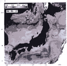A satellite thermal image of SST around Japan, obtained by the NOAA/AVHRR on 12 June 1986.
Issued from : T. Sugimoto & H. Tameishi in Deep-Sea Res., 39, suppl. 1, 1992. [p.S186, Fig.1 (a)].

 

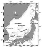The bottom topography and geographical locations for the Japan/East Sea. The depth contours are at 300 and 1000 m.
Issued from : D.-K. Lee & P.P. Niiler in Deep-Sea Res. II, 52, 2005. [p.1548, Fig.1].

 

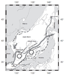Schematic map of the surface currents in the Japan/East Sea based on Lee and Niiler's (2005) drifter observations. Dotted paths (Tsushima Warm Current [TWC] and North Korean Cold Current [NKCC]) represent the currents observed only during spring and summer, and solid paths (East Korean Warm Current [EKWC] and East Sea Current) represent the currents observed all the year.
Issued from : D.-K. Lee & P.P. Niiler in Deep-Sea Res. I, 57, 2010. [p.1223, Fig.1].

 

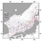Mean velocity and variance ellipses on 0.5^° x 0.5^° bins. Red vectors are for the mean speed larger than 10 cm/s and blue vectors are those smaller than 10 cm/s.
Issued from : D.-K. Lee & P.P. Niiler in Deep-Sea Res. II, 52, 2005. [p.1550, Fig.3].

 

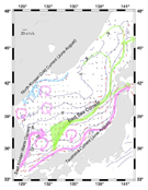The schematic patterns of surface circulation from drifter observation drawn on 100 m mean temperature from JMA (2001) [In Oceanographic Normals and Analysis for the period 1971–2000 (CD-ROM). Japan Meteorological Agency, Tokyo]. Red vectors are for mean current larger than 10 cm/s.
Issued from : D.-K. Lee & P.P. Niiler in Deep-Sea Res. II, 52, 2005. [p.1560, Fig.16].

 

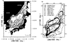Bathymetry of the Japan Sea (a) and numbers show the water depth in meters.In (b) schematic map for sea surface currents (after Senjyu, 1999) with abbrevations: TWC = the Tsushima Warm Current; LC = the Liman Current; EKWC = the East Korean Warm Current; NKCC = the North Korean Cold Current;
OI : the Oki Island and NP : Noto Peninsula.
Issued from : A. Morimoto & T. Yanagi in J. Oceanogr., 2001, 57. [p.2, Fig.1].

Issued from : M.-C. Jang, S.H. Baek, P.-G. Jang, W.-J. Lee & K. Shin in Ocean and Polar Res., 2012, 34 (1). [p.40, Fig.2].
Weekly average sea surface temperature (SST) derived from NOAA/AVHRR during periods in February and July 2009 in the Korea Strait.
Sampling stations are marked as circles.

Issued from : L.-C. Tseng, R. Kumar, H.-U. Dahms, Q.-C. Chen & J.-S. Hwanh in Zool. Studies, 2008, 47 (1). [p.53, Fig.4].
Monthly average sea-surface temperatures (SSTs) derived from averaged hourly recordings (AVHRRs) for (A) Aug. 1998, (B) Dec. 1998, (C) Mar. 1999, and (D) May 1999.

Nota: The Taiwan Strait is a relatively shallow (with an average depth of 60 m), 350 km long, and 180 km wide channel between the island of Taiwan and the southeastern Chinese coast, connecting the two marginal seas of the western Pacific, the East China Sea and the South China Sea.
In the Taiwan Strait there is a congruence of 3 different water masses (East China Sea, South China Sea), and the water masses representing the Kuroshio Current of the western North Pacific. Such hydrographic conditions affect the zooplankton community composition in the Taiwan Strait.
Wind patterns in this region are determined by the typical East Asian monsoon that is from the northeast (NE) during winter (Oct.-Mar.) and from southwest (SW) during summer (May-Aug.).
During the NE monsoon the China Coastal Current with low temperatures, low salinities, and high nutrient levels moves southwards driving zooplankton from the Bohai Sea, the Yellow Sea, and the East China Sea towards the Taiwan Strait.
Throughout the year, the warm, highly saline, and nutrient-poor Kuroshio Branch Current intrudes into the Taiwan Strait through the northern South China Sea and along the coast of southwestern Taiwan. However, during the prevailing NE monsoon period, the southherly flowing China Coastal Current near the Penghu Channel, south of the Changyun Ridge in the southeastern Taiwan Strait.
In spring when the NE monsoon weakens the Kuroshio Branch Current moves northward along the local isobaths into the northern part of the Taiwan Strait. Conversely, under the prevailing winds of the SW monsoon (May-Aug.), the South China Sea Warm Current with intermediate temperatures, salinities, and nutrient levels intrudes into the Taiwan Strait and moves northward together with the Kuroshio Branch Current that transports plankton from the northern South China Sea.
The hydrographic properties of this part (NW Taiwan) of the Taiwan Strait are mainly influenced by the NE and SW monsoons. The influence of cold water masses disappears during summer with increasing strength of the SW monsoon as water masses from the northern part of the South China Sea enter the Taiwan Strait and influence the fhydrography around the west coast of Taiwan, and Guangdong and Fujian Provinces, China.

The Japan Current or Kuroshio:
The branch of the North Equatorial Current that flows Northwestward reaches Taiwan, and from there the Japan Current takes on a clearly defined identity.
Off Taiwan, the Kuroshio is 100 miles wide with a speed of 1.5 knots. Further North, along the Ryukyu Islands, its width decreases to about sixty miles; its speed is then 2 to 3 knots in the axis, and 1 knot at the edges. At 32° North, off Kyushu Island, the Kuroshio's speed does not exceed 2 knots. At Cape Moroto Saki, beyond which the Japanese coast turns sharply Northward, the current is 50 miles wide; its speed, averaging 2 knots, can sometimes reach 5 knots. The current then turns Eastward, merging with the eastward drift of the North Pacific.
In winter, the surface waters of the Kuroshio have a temperature of about 24° off Taiwan; this temperature decreases progressively Northward, falling to about 13°C at 35° latitude. In summer, these temperatures are about 27° and 18°C respectively; it is only in this season that the Kuroshio waters are clearly warmer than the surrounding open-sea waters. Throughout its course, the Kuroshio has a salinity of 34.5. Its waters are dark blue (its name means "black current" in Japanese).

Sea of Japan Current:
A branch of the Kuroshio enters the Sea of Japan through the Korea Strait (also called the Tsushima Current); it has an average speed of 1.5 knots, stronger in summer, when its speed exceeds 2.5 knots. The current turns Northeastward in the Sea of Japan, runs along the Japanese coast at a speed of 10 miles per day, and reaches the Gulf of Tartary. Along the Asian coast, there is a southward current, more pronounced in winter than in summer.
In the Tsugaru and La Pérouse Straits, the current flows Eastward, often at very high speeds, reaching 6 to 7 knots.

Oyashio Current:
A cold current coming from the Bering Sea, the Oyashio, flows Southward at a speed of more than 1 knot along the Kuriles and as far as the shore of Honshu, where it creates, in contrast with the Kuroshio which spreads further offshore, a sort of contact zone. This current never reaches the approaches to Tokyo Bay; the negative temperature anomalies observed there in winter are due to upwellings of cold water, or to the influence of the low temperatures then prevailing in Japan.

References:
J. Rouch, Traité d'Océanographie physique. Les mouvements de la mer. Vol. 3. Édit. Payot, Paris, 1948.
National Geographic Society, Washington D.C., 1981
Atlas of Pilot Charts http://msi.nga.mil/NGAPortal/MSI.portal?_nfpb=true&_pageLabel=msi_portal_page_62&pubCode=0003 NATIONAL GEOSPATIAL-INTELLIGENCE AGENCY (USA)

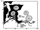Schematic diagram for the transport of the fresh Oyashio water (black arrowed curves) and old NPIW (North Pacific Intermediate Water) (gray arrowed curves) in the salinity minimum layer.
The movement and mixing of these waters were strongly related to the small and meso scales features in the MWR (Mixed Water Region) such as the First Branch of the Oyashio (FBO), the Second Branch of the Oyashio (SBO), the inner cold belt (ICB), warm core ring (WCR) and warm streamer (WS).
Old NPIW transported by the Kuroshio Extension (KE) strongly mixed with the fresh Oyashio water extended from the first branch of the Oyashio (FBO) in and around WS.
The fresh Oyashio water extended from SBO was transported eastward along the northern edge of KE beyond 150°E with a form of rather narrow band.
The subsurface intrusion at the northern edge of KE ejected lens-like Oyashio waters southward across KE axis and split northwarde into a warm core ring probably by the interaction of KE and WCR, suggesting the processes of freshening NPIW in the offshore MWR and the Kuroshio recirculation region.
The aim is to understand the actual formation process of the North Pacific Intermediate Water examined on the basis of a synoptic CTD observation carried out in May-June 1992.
Issued from : K. Okuda, I. Yasuda, Hiroe Y. & Y. Shipmizu in J. Oceanogr., 2001, 57. [p.138, Fig.10].

233 species are common to Japan and the sub-Arctic zone (i.e. 32.4 %), although the dominant influence on Japanese planktonic fauna is generally tropical.

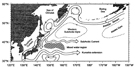Diagram of the relationship of the Oyashio Current to other currents in the northwest Pacific Ocean (Modified from Qiu, 2001).
Issued from : Y. Sakurai in Deep-Sea Research II, 2007, 54; [p.2527, Fig.1].

Of 172 species common to the NW and NE Pacific sub-Arctic zones, 11 are known only in these two zones.

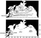Schematic current systems (top, redrawn from Favorite & al., 1976) and sampling stations in the subarctic Pacific Ocean and neighboring waters (bottom).
Issued from : T. Kobari & T. Ikeda in J. Plankton Res., 2001, 23 (3). [p.288, Fig.1].

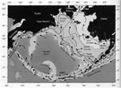The Bering Sea. Isobaths shown are 50 m (between inner and middle domains), 100 m (between middle and outer domains) and 200 m (between outer domain and slope/basdin. Schematic of major currents based on Stabeno & al. (1999). AC: Anadyr Current; ACC: Alaska Coastal Current; ANSC: Aleutian North Slope Current; BS: Bering Strait.
Issued from : K. Aydin & F. Mueter in Deep-Sea Research II, 2007, 54. [p.2502, Fig.1].

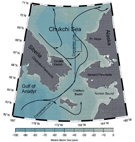Map of the northern Bering Sea and Chukchi.
The box marks the survey area of the hydrographic conditions (temperature, salinity and chlorophyll) and Gray whale counts during June to September. The arrows show the prevailing current regime.
Issued from : B.A. Bluhm, K.O. Coyle, B. Konar & R. Highsmith in Deep-Sea Resaeach, 2007, 54. [p.2921, Fig.1]. .

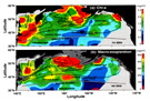Average summer season distributions of upper ocean chlorophyll concentration (upper panel) and zooplankton biomass (lower panel) in the subarctic Pacific, overlaid with circulation pattern. Figure courtesy of K. Tadokoro, modified by colorization and addition of circulation streamlines from Sugimoto and Tadokoro, 1997.
Issued from : Mackas D.L. & Tsuda A., 1999. - Mesozooplankton in the eastern and western subarctic Pacific: community structure, seasonal life histories, and interannual variability. Progress in Oceanography, 43. [p.352, Fig.8].

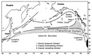Map of the subarctic Pacific showing place names referred to in this paper (adapted from Brodeur et al., 1996).
Issued from : Mackas D.L. & Tsuda A., 1999. - Mesozooplankton in the eastern and western subarctic Pacific: community structure, seasonal life histories, and interannual variability. Progress in Oceanography, 43. [p.337, Fig.1].

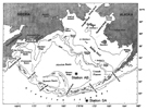Major topographic features of the Bering Sea and Aleutian Islands. Contours of 100, 200, 1000 and 3500 m are shown. (Basic map from U.S. GLOBEC 1996).
Issued from : Takahashi K., 1998. - The Bering and Okhotsk Seas: modern and past paleoceanographic changes and gateway impact. Journal of Asian Earth Sciences, 16 (1). [p.50, Fig.1].

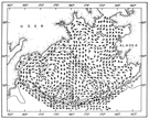A map showing surface currents in the Bering Sea (from Arsen'ev 1967).
Issued from : Takahashi K., 1998. - The Bering and Okhotsk Seas: modern and past paleoceanographic changes and gateway impact. Journal of Asian Earth Sciences, 16 (1). [p.51, Fig.2].

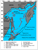Surface thermal fronts of the Okhotsk Sea from Pathfinder data, 1985–1996.
Issued from : Belkin I.M. & Cornillon P.C., 2004. - Surface Thermal Fronts of the Okhotsk Sea. Physical Oceanography, 2 (1-2). [p.9, Fig.1].

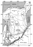Major topographic features of the Okhotsk Sea and Kuril Islands. Contours of 100, 200, 500, 1000, 2000, 2500 and 3000 m are shown (modified from Gnibidenko and Khvedchuk 1982).
Issued from : Takahashi K., 1998. - The Bering and Okhotsk Seas: modern and past paleoceanographic changes and gateway impact. Journal of Asian Earth Sciences, 16 (1). [p.52, Fig.3].

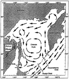A map sho wing surface currents in the Okhotsk Sea and adjacent regions. Note that a part of the Kamchatka Current enters into the Okhotsk Sea and a part of the Okhotsk Gyre water exits from the Sea to the Pacific to form the Oyashio Current just south of the Kuril Islands. The Okhotsk Sea circulation is compiled by R. Tiedemann, employing data obtained by Dodimead et al. (1963), Sancetta (1981), and Talley (1991).
Issued from : Takahashi K., 1998. - The Bering and Okhotsk Seas: modern and past paleoceanographic changes and gateway impact. Journal of Asian Earth Sciences, 16 (1). [p.53, Fig.4].

Kamchatka Current:
This cold current, coming from the Bering Sea, flows along the eastern coast of the Kamchatka Peninsula and the Kuril Islands as far as Hokkaido, where it merges with the Oyashio.

Currents of the Sea of Okhotsk:
The general movement of the currents is anticyclonic, following the coastlines.
Along the northern coast, there is a westward current; along the western coast and near Sakhalin Island, a southward current; along the coast of Kamchatka, a northward current. The southward currents are on the whole predominant; they are weak, barely reaching a speed of half a knot, and are often strongly modified by tidal currents, whose diurnal component has a large amplitude: at the entrance to the Gulf of Penzhina, these tidal currents reach speeds of 6 to 7 knots. In the channels separating the Kuril Islands, the currents, strongly influenced by the tides, are very fast (speeds exceeding 6 knots have often been observed).
In general, the currents flow Southward, carrying the cold waters of the Sea of Okhotsk to the Oyashio.

References:
J. Rouch, Traité d'Océanographie physique. Les mouvements de la mer. Vol. 3. Édit. Payot, Paris, 1948.
National Geographic Society, Washington D.C., 1981
Atlas of Pilot Charts http://msi.nga.mil/NGAPortal/MSI.portal?_nfpb=true&_pageLabel=msi_portal_page_62&pubCode=0003 NATIONAL GEOSPATIAL-INTELLIGENCE AGENCY (USA)

 

Zones: North East Pacific(24) ; California (25)

	24	25
Total species:	298 (11.6 %) (+ 1 ind.)	458 (17.8 %) (+ 1 ind.)
Calanoida:	231	360
other orders	67	98

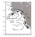Map of the NE Pacific (adapted from Ware and McFarlane, 1989) showing location of the shelf-slope-offshore transition region (shaded area) and annual-averaged large-scale current patterns (arrows). The coastal transition region includes both the NE Pacific alongshore boundary current systems: the equatorward/upwelling California Current and the poleward/downwelling Alaska Current/Alaska Coastal Current. Although not shown in the annual averages, the boundary currents undergo seasonal variability in speed and direction (generally more poleward/less equatorward in winter, more equatorward/less poleward in summer), and both produce strong mesoscale cross-shore motion in the form of meanders, eddies and filaments.
Issued from : Mackas D.L. & Coyle K.O., 2005. - Shelf-offshore exchanges processes, and their effects on mesozooplankton biomass and community composition patterns in the northeast Pacific. Deep-Sea Res. II , 52. [p.708, Fig.1].

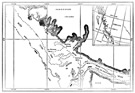Map of the study area showing bathymetry and approximate summer circulation pattern. Solid arrows indicate near-bottom currents, open arrows show upper layer currents.
Issued from : Mackas D.L. & Sefton H.A., 1982. - Plankton species assemblages off southern Vancouver Island: Geographic pattern and temporal variability. Journal of Marine Resarch, 40 (4). [p.1176, Fig.1].

The north-eastern Pacific (Aleutians , Gulf of Alaska , "P" Station, British Colombia), sub-Arctic in character, is one of the least diversified regions.

It is, however, also one of the least explored (Wilson, 1942 a, 1950; Davis, 1949) with the exception of "P Station" (50° N, 145° W). In this region, 175 species are shared with the Californian zone (i.e. 58.5 %) and 172 species with the North-west region (i.e. 57.5 %). These percentages confirm the uniqueness of the sub-Arctic community.

The communities of the Californian and Japanese regions have been united in the northern sub-tropical zone (Van der Spoel & Heyman, 1983, p.12, fig.11), which would seem to confirm the percentages of species common to the two zones: 333 common species (i.e. 72.5 %).

Alaska Current:
The North Pacific Drift, when it reaches the American shores at around 50° latitude, splits into two currents. To the North, the Alaska Current follows the coast of British Columbia and Alaska Northwestward at a speed that can reach 1.5 knots. It rounds the Gulf of Alaska, describing a counter-clockwise circuit, and strengthens west of Kodiak Island as far as the easternmost Aleutian Islands. These waters are warmer than those further South.

California Current:
The second branch of the North Pacific Drift follows the American coast Southward from latitude 50° North to the Baja California peninsula at 23° North. It is a cold current, 200 to 300 miles wide, with a speed of about a quarter of a knot. Accompanied by upwelling of cold water, it produces, at the entrance to San Francisco Bay, sea temperatures that do not exceed 15°C even at the height of summer.
The current follows the direction of the coast Southeastward, but begins to bend Southward and Southwestward from the latitude of Monterey onward. Along the coast there is then, especially in winter, a countercurrent known as the Davidson Current.
Off Cape San Lucas, the southern tip of Baja California, the California Current turns Southwestward and joins the waters of the Equatorial Current.

References:
J. Rouch, Traité d'Océanographie physique. Les mouvements de la mer. Vol. 3. Édit. Payot, Paris, 1948.
National Geographic Society, Washington D.C., 1981
Atlas of Pilot Charts http://msi.nga.mil/NGAPortal/MSI.portal?_nfpb=true&_pageLabel=msi_portal_page_62&pubCode=0003 NATIONAL GEOSPATIAL-INTELLIGENCE AGENCY (USA)

 

Zones: Central Tropical Pacific (19) ; Eastern Tropical Pacific (20)

	19	20
Total species:	541 (21.1 %) (+ 9 ind.)	514 (20 %) (+ 3 ind.)
Calanoida:	433	401
other orders	108	113

352 species species are common to the two regions (i.e. 64 % and 68.1 % respectively).

Zone 19:

In the region between the tropics, subject to the trade winds, the waters of the North Pacific Ocean have a general westward movement. Two equatorial currents are thus formed.
The North Equatorial Current lies between the parallels 20°-25° North and 8°-9° North. The South Equatorial Current lies between the parallels 4°-5° North and 20°-25° South.
The Hawaiian Islands lie within the North Equatorial Current, and Tahiti within the South Equatorial Current, at its southern limit.
The speed of these equatorial currents varies between half a knot and 3 knots; it decreases with distance from the equator. The South Equatorial Current has a stronger speed than the North Equatorial Current.

The two equatorial currents do not merge, as they do in the Atlantic, but are separated throughout their course by an eastward countercurrent that is felt from south of the Philippines to the American coast, over a band 300 miles wide, between 4°-5° North latitude and 8°-9° North latitude in the Northern Hemisphere summer, and over a much narrower band in winter, mainly in the middle of the Pacific Ocean and further South. The speed of the countercurrent is weaker than that of the equatorial currents, not exceeding 2 knots. During the Northern Hemisphere winter months, it can become barely perceptible. The countercurrent accounts for, to a greater extent than in the Atlantic, the eastward return of the waters carried by the equatorial currents.
The presence of archipelagos along the course of the equatorial currents brings about modifications, though only local ones, splitting the currents and sometimes strongly deflecting them. Upwelling of deep water results in a drop in surface temperature.
In the eastern part of the Pacific Ocean, between the Galápagos and the Gulf of Panama, a region where the trade wind is not yet well established and where monsoons and variable winds prevail, marine circulation is very confused. On the whole, stagnant waters are found there, which probably take little part in the general circulation, and whose temperature is often very high.
On reaching the vicinity of the Philippines, at about 10° North latitude, the North Equatorial Current splits into two branches; one heads Northwestward to join the Japan Current, and the other, turning Southward, runs along the eastern coast of Mindanao at a speed of 2 knots, before joining the waters of the equatorial countercurrent.

The North Pacific Drift:
The main branch of the Kuroshio, which turns Eastward around latitudes 35° to 40° North, rapidly loses speed as it moves away from Japan. Its limits become uncertain both to the North and to the South. It is no longer a true current, but a drift, which, from the 180° meridian onward, does not exceed a speed of 12 miles per day.
By the time the Kuroshio merges with the slower drift driven by the westerly winds, it is much narrower, shallower and overall cooler. From the point where the Kuroshio merges with the North Pacific Drift to the western coast of America, the distance is 3500 miles; thus the thermal influence of the Kuroshio on the northern shores of the Pacific is greatly reduced, though not negligible: the coastal regions of southern Alaska, at latitudes of 60°, have winter temperatures barely below 0°C, whereas at the same latitude the coastal regions of Kamchatka have temperatures of -15° to -20°C.

Drift of the South Pacific waters:
Between the parallels of 40° and 50° South, under the influence of the westerly winds very frequent at these latitudes, there is, if not a true current, at least a drift flowing Eastward as far as the coasts of Chile. Its speed is very low, on the order of a few miles per day; it is stronger west of the 120° West meridian, especially during the austral winter, when speeds of 1 knot have been observed.
The limits of this drift are marked by the subpolar convergence line around 55° South and the subtropical convergence line around 35° South. The southern part of the drift tends to flow Southeastward, the northern part Northeastward.

References:
J. Rouch, Traité d'Océanographie physique. Les mouvements de la mer. Vol. 3. Édit. Payot, Paris, 1948.
National Geographic Society, Washington D.C., 1981
Atlas of Pilot Charts http://msi.nga.mil/NGAPortal/MSI.portal?_nfpb=true&_pageLabel=msi_portal_page_62&pubCode=0003 NATIONAL GEOSPATIAL-INTELLIGENCE AGENCY (USA)

 

Zones: E. Australia - New Zealand (18) ; Chile (sensu lato) (26)

	18	26
Total species:	534 (20.8 %) (+ 15 ind.)	436 (17 %) (+ 1 ind.)
Calanoida:	400	357
other orders	134	79

Major currents and circulation patterns around Australia.
The continent is bounded by the pacific ocean to the east, the indian Ocean to the west and the Southern Ocean to the south.
Issued from : E.S. Poloczanska & al. in Oceanography and Marine Biology: An Annual Review, 2007, 45. [p.409, Fig.2]. Figure courtesy of S. Condie/CSIRO.

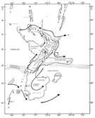Major bathymetric features of the New Zealand region, surface currents, place names, and topographic features.
Issued from : Bradford J.M., Roberts P.E., 1978. - Distribution of reactive phosphorus and plankton in relation to upwelling and surface circulation around New Zealand. New Zealand Journal of Marine and Freshwater Research, 12 (1): [p.3, Fig.1].

388 species are common to the Indian Ocean and the E. Australia - New Zealand zone.

Australian currents:
Off the Samoa Islands, the South Equatorial Current appears to split into two branches: one continues Westward to New Guinea, where the currents are strongly influenced by the monsoon. During the Northern Hemisphere summer, a fairly strong current flows Westward and Northwestward, whereas in winter a weak eastward current is observed.
Between New Guinea, the Solomon Islands, Australia and New Caledonia, the currents are confused, weak and variable according to the season. Thus, in the Torres Strait, in December, January and February, the current flows Eastward; it flows Westward for the rest of the year. This current can become fast when the wind is strong and blows in the same direction. Similarly, on the Australian coast north of Brisbane, a Southeastward current is observed in winter (Northern Hemisphere), and a Northwestward current in summer.
The second branch of the equatorial current, after crossing the Fiji Archipelago, passes south of New Caledonia and reaches the Australian coast off Brisbane. It then forms the East Australian Current proper, which runs along the coast at a distance of 20 to 60 miles, without extending offshore as far as the Middleton and Elizabeth Reefs, nor Lord Howe Island. The East Australian Current flows Southward at a speed of 0.5 to 3 knots, reaching up to 4 knots in places. Close to shore, there is often a countercurrent flowing Northward.
The East Australian Current turns Southeastward off Sydney, and between Australia and New Zealand a vast counter-clockwise circuit takes shape.
References:
J. Rouch, Traité d'Océanographie physique. Les mouvements de la mer. Vol. 3. Édit. Payot, Paris, 1948.
National Geographic Society, Washington D.C., 1981
Atlas of Pilot Charts http://msi.nga.mil/NGAPortal/MSI.portal?_nfpb=true&_pageLabel=msi_portal_page_62&pubCode=0003 NATIONAL GEOSPATIAL-INTELLIGENCE AGENCY (USA)

254 species are common to the two southern Pacific zones (i.e. 46.3 % and 58.1 % respectively).

The Peru Current or Humboldt Current:
The South Pacific Drift, on approaching the coasts of Chile, splits into two branches at around the 50th degree of South latitude.
The first, known as the Cape Horn Current, carries waters around Tierra del Fuego at a speed of 1 knot, at a temperature higher than that of the Falklands Current at the same latitude.
The second branch, the Peru or Humboldt Current, flows Northward. It is observed mainly from Valdivia (40° South) to Cape Blanco (4°30'S).
The Peru Current has an average width of only 100 to 150 miles. Its speed, stronger off the Peruvian coast than off the Chilean coast, barely exceeds half a knot on average. It is chiefly recognisable by its low temperature, 15° to 19°, several degrees lower than the surface temperature observed offshore at the same latitude, and sometimes as much as ten degrees lower than the air temperature at sea level. It is also particularly rich in phosphates and nitrates.
Humboldt attributed these low temperatures to a cold current coming from the Antarctic regions. These low surface water temperatures are attributed to upwelling of deep water along the steeply sloping coasts. Salinity measurements made by Sverdrup (1930) show that the waters do not originate from very deep layers, but from no deeper than 300 metres.
The waters of the Peru Current are less saline than the offshore waters, and are also distinguished by their richness in phytoplankton, which gives them a green colour, contrasting with the indigo blue of the open sea. The Peru Current is subject to significant variations that bring it closer to, or further from, the coast. In its northern part its limits are variable. A southward current, called El Niño, which occurs north of Cape Blanco, especially at the height of the austral summer (around Christmas), sometimes extends as far as 12° or 15° South latitude, causing the cold coastal waters to disappear and turning the dry coastal climate into a rainy one for a few weeks. When this phenomenon occurs, this influx of warm water from the West temporarily causes the Humboldt Current to disappear or be pushed offshore.
References:
J. Rouch, Traité d'Océanographie physique. Les mouvements de la mer. Vol. 3. Édit. Payot, Paris, 1948.
National Geographic Society, Washington D.C., 1981
Atlas of Pilot Charts http://msi.nga.mil/NGAPortal/MSI.portal?_nfpb=true&_pageLabel=msi_portal_page_62&pubCode=0003 NATIONAL GEOSPATIAL-INTELLIGENCE AGENCY (USA)

 

Zones: South Africa (E & W), Namibia (5) ; Gulf of Guinea (sensu lato) (6)

	5	6
Total species:	288 (11.2 %) (+ 3 ind.)	371 (14.4 %) (+ 2 ind.)
Calanoida:	235	289
other orders	53	82

Of the "endemic" to South Africa , 9 species are on the Atlantic side and 2 in the Indian Ocean (Acartia (Acartia) longisetosa, Acartia (Acartia) nana, Centropages natalensis, Centropages tenuicornis, Diaixis centrura).

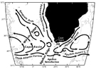A conceptual diagram of the circulation of intermediate water in the eastern South Atlantic and around southern Africa (adapted from Boebel et al., 1998 and based on the work of Shannon and Nelson, 1996; Reid, 1989; and others). AB refers to the Agulhas Bank, and AP to the Agulhas Plateau.
Issued from : Richardson P.L., Lutjeharms J.R.E. & Boebel O., 2003. - Introduction to the "Inter-ocean exchange around southern Africa". Deep Sea Research II, 50 (1): [p.5, Fig.2].

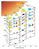Inverse model mass transport (in Sv) and standard errors for the Agulhas Current system for the LADCP experiment.
Net mass transport values are displayed on the top, and each individual layer displays the mass transport associated with it. Red arrows represent diapycnal transports, and blue, yellow, and orange arrows represent isopycnal transports. Small circular arrows indicate the location of some of the sampled eddies. PE refers to Port Elizabeth (36°S). EL refers to East London (34°S). PS refers to Port Shepstone (32°S). RB refers to Richards Bay (30°S).
Issued from : Casal T.G.D., Beal L.M., Lumpkin R. & Johns W.E., 2009. - Structure and downstream evolution of the Agulhas Current system during a quasi-synoptic survey in February-March 2003. Journal of Geophysical Research, 114 (C03001): [p.6, Fig.2].

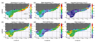Physical oceanography during the survey. (a) Temperature at 7 m; (b) salinity at 7 m; (c) mean temperature; (d) mean salinity; (e) integrated chlorophyll a; and (f) mean oxygen. Means and integration are over the water column. Visualization performed in Ocean Data View software (Schlitzer, 2008).
Issued from : Lebourges-Dhaussy A., Coetzee J., Hutchings L., Roudaut G. & Nieuwenhuys C., 2009. - Zooplankton spatial distribution along the South African coast studied by multifrequency acoustics, and its relationships with environmental parameters and anchovy distribution. ICES Journal of Marine Science, 66. [p.1057, Fig.2].

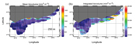Horizontal distribution of the global zooplankton. (a) Mean biovolume (mm³ m^-3); (b) integrated biovolume (mm³ m^-2).
Issued from : Lebourges-Dhaussy A., Coetzee J., Hutchings L., Roudaut G. & Nieuwenhuys C., 2009. - Zooplankton spatial distribution along the South African coast studied by multifrequency acoustics, and its relationships with environmental parameters and anchovy distribution. ICES Journal of Marine Science, 66. [p.1058, Fig.4].

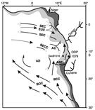Atlantic currents west of Africa.
AC = Angola Current, ABF = Angola Benguela Front, BCC = Benguela Coastal Current, BOC = Benguela Oceanic Current, SECC = South Equatorial Counter Current, SEC = South Equatorial Current, EUC = Equatorial Undercurrent
Issued from : Hogan C., 2012. - Angola-Benguela Front. Retrieved from http://www.eoearth.org/view/article/150063

Zones : Central South Atlantic (12) ; Brazil-Argentina (SW Atlantic) (13)

	12	13
Total species:	337 (13.1 %) (+ 3 ind.)	397 (15.5 %) (+ 3 ind.)
Calanoida:	291	278
other orders	46	119

183 species are common to the two zones. It is important to note that most of our knowledge of the diversity of Copepoda in the central South Atlantic comes from very old studies (e.g. Wolfenden, 1911).

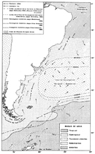Hydrology from Southwest Atlantic Ocean.
Issued from : E. Boltovskoy in Atlas del Zooplancton del Atlántico sudoccidental, 1981, ed. D. Boltovskoy, Publ. special des INIPED, Mar del Plata, Argentina. [p.230, Fig.131].

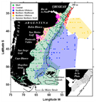
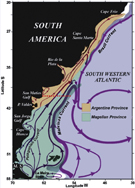Schematic ocean circulation of the southwestern South Atlantic (modified from Matano et al., 2010) and continental shelf biogeographic provinces (background shading, modified from Balech and Ehrlich (2008) and Boschi (2000)).
The red dotted line represents the boundary between the provinces from Spalding et al. (2007), referred to by those authors as Warm Temperate Southwestern Atlantic and Magellan provinces. M.S.= Magellan Strait.
For interpretation of the references to color in this figure legend, the reader is referred to the web version.
Issued from : E.M. Acha, M.D. Viñas, C. Derisio, D. Alemany & A.R. Piola inJ. Mar. Syst., 2020, Volume 204 (103281). [Fig.1].

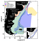Ecoregions and marine fronts at the southwestern South Atlantic.
Blue lines represent fronts associated with the boundaries of the ecoregions.
A = Plata plume front (33.5 surface isohaline, Piola & al., 2008; Piola & al., 2005).
B = Subtropical front and Brazil-Malvinas Confluence (35 surface isohaline, Piola & al., 2000).
C = Patagonian shelfbreak front (maximum SST gradient for January, Piola & Falabella, 2009).
D = Shallow sea front (Simpson's parameter critical value for summer phyC = 40 J m-3, Bianchi & al., 2005).
E = Estuarine front of Rio da la Plata (27.5 surface isohaline for November-March, Guerrero & al., 2010).
For interpretation of the references to color in this figure legend, the reader is referred to the web version.
Issued from : E.M. Acha, M.D. Viñas, C. Derisio, D. Alemany & A.R. Piola inJ. Mar. Syst., 2020, Volume 204 (103281). [Fig.7].

Ecoregions based on copepod's presence/absence data. Map of the sampling stations assemblages defined by cluster and MDS analysis.
Large-scale patterns of pelagic copepods: Occurrence percentage of species expressed in Table 3 and indicator species for each ecoregion in Table 5. .
Issued from : E.M. Acha, M.D. Viñas, C. Derisio, D. Alemany & A.R. Piola inJ. Mar. Syst., 2020, Volume 204 (103281). [Fig.3].

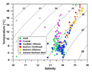Relationships of the ecoregions with water masses. Sampling stations assemblages defined by CLUSTER and MDS analyses in a temperature-salinity (T/S) space.
Temperature and salinity climatological data from the World Ocean Atlas.
For interpretation of the references to color in this figure legend, the reader is referred to the web version.
Issued from : E.M. Acha, M.D. Viñas, C. Derisio, D. Alemany & A.R. Piola inJ. Mar. Syst., 2020, Volume 204 (103281). [Fig.4].

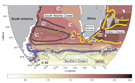The oceanic circulation around the Agulhas choke point and location of Tara Oceans stations.
The map shows the location of sampling stations, together with trajectories of the young and old Agulhas rings (TARA_068 and TARA_078, red and green tracks, respectively).The stations here considered as representative of the main basins are (i) TARA_052, TARA_064, and TARA_065 for Indian Ocean; (ii) TARA_070, TARA_072, and TARA_076 for the South Atlantic Ocean, and (iii) TARA_082, TARA_084, and TARA_085 for the Southern Ocean.The mean ocean circulation is schematized by arrows (currents) and background colors [surface climatological dynamic height (0/2000 dbar from CARS2009; www.cmar.csiro.au/cars)] (70). Agulhas rings are depicted as circles.
Issued from : Villar E., Farrant G.K, Follows M. & al. in Science, 2015, 348 (6237). [p.2, Fig.1].

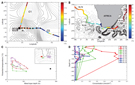Properties of the young Agulhas ring (TARA_068).
(A) Daily sea surface height around young Agulhas ring station TARA_068 [absolute dynamic topography (ADT) from www.aviso.altimetry.fr]. R, C1, and C2, respectively, denote the centers of the Agulhas ring and two cyclonic eddies. The contour interval is 0.02 dyn/m. The ADT values are for 13 September 2010. Light gray isolines, ADT < 0.46 dyn/m. The crosses indicate the CTD stations, and the square symbol indicates the position of the biological station TARA_068. The biological station coincides with the westernmost CTD station. ADT is affected by interpolation errors, which is why CTD casts were performed at sea so as to have a fine-scale description of the feature before defining the position of thebiological station (23). Superimposed are the continuous underway temperatures (°C) from the on-board thermosalinograph.
(B) Same as (A) but at the regional scale. Round symbols correspond to biological sampling stations.The contour interval is 0.1 dyn/m.
(C) Seasonal distribution of the median values of the mixed layer depths and temperatures at 10 m (from ARGO) provided by the IFREMER/LOS Mixed Layer Depth Climatology L2 database (www.ifremer.fr/cerweb/deboyer/mld) updated to 27 July 2011.The mixed layer is defined using a temperature criterion. The star symbol represents the young ring station TARA_068. (Inset) Geographic position of the areas used to select the mixed layer and temperature data. The mixed layer depth measured at TARA_068 is outside the 90th percentile of the distribution of mixed layer depths for the same month for both the subtropical (red and magenta) regions.The temperature matches the median for the same month and region of sampling.
(D) Nitrite (NO₂) concentrations from CTD casts at different sampling sites (expressed in mmol/m³).
Issued from : Villar E., Farrant G.K, Follows M. & al. in Science, 2015, 348 (6237). [p.5, Fig.4].

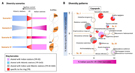Plankton diversity patterns.
(A) Schematic representation of four scenarios of diversity patterns between the Indian and South Atlantic basins (I to IV): Plankton is transported from the Indian Ocean (pink, right) to the South Atlantic Ocean (blue, left) through the choke point (red, CP). The thickness of each colored section represents the level of diversity specific to each region. The observed percentage of V9 rDNA OTUs corresponding to each scenario is indicated in the pie charts to the left (out of 1063 OTUs of the full V9 rDNA barcode data set).
(B) V9 rDNA OTU diversity patterns for copepods. Each circle on the charts represents a V9 rDNA OTU plotted with coordinates proportional to ribotypes specific to the Indian Ocean (x axis) and the South Atlantic Ocean (y axis). For instance, the copepod Acartia negligens in the top right corner of sector II corresponds to the "bow tie" scenario II of (A) (i.e., a copepod with representative V9 rDNA barcodes in both Indian and South Atlantic Oceans, the vast majority of which are specific to their respective ocean basin). In contrast, the majority of barcodes for Sinocalanus sinensis in sector III are found in both Indian and South Atlantic Oceans [cosmopolitan OTU corresponding to the "Everything is everywhere" flat diversity diagram of (A), scenario III]. If more than 10 barcodes were found in the young Agulhas ring (TARA_068), their distribution is indicated in a pie chart (colors are coded in the legend inset); otherwise, the OTUis represented by an empty circle. Circle sizes are proportional to the number of considered barcodes for each OTU.
Issued from : Villar E., Farrant G.K, Follows M. & al. in Science, 2015, 348 (6237). [p.6, Fig.5].

 

Zones: North-East Atlantic (8) ; Mediterranean - Black Sea (14) :

	8	14
Total species:	746 (29 %) (+ 14 ind.)	587 (22.9 %) (+ 1 ind.)
Calanoida:	591	388
other orders	155	199

The Canary Current:
East of the Azores meridian, the Atlantic Ocean drift following on from the Gulf Stream becomes increasingly confused. It splits into two branches west of the English Channel. One flows Northward along the coast of Ireland; the other enters the Bay of Biscay.
On 8 February 1892, Prince Albert of Monaco presented to the Academy of Sciences a map of North Atlantic currents showing a clockwise current, flowing Southward along the coasts of France and Westward along the coasts of Spain.
The current felt between the Azores and the western coasts of Spain, Portugal and the African coast as far as the Cape Verde Archipelago generally flows Southward or Southwestward. To the North it is known as the Portugal Current; its speed averages 2 miles per day in winter and 3 miles per day in summer. From the latitude of Cape St. Vincent (Portugal) to the latitude of Cape Blanc (Mauritania), the southward current is known as the Canary Current. Its direction is Southward, or South-Southwestward, as far as the latitude of Cape Juby (28° N Lat.: Canary Islands); it then turns further Southwestward. Its speed is stronger in its southern part and can reach 2 knots or more in the vicinity of Cape Juby, when well-established North and Northwest winds blow; but on average it does not exceed half a knot, being slightly stronger in summer than in winter. Southwest winds can temporarily suppress the southward current.
The Canary Current is a cold current, partly originating from more northerly latitudes, partly fed by upwelling of deep water along the coasts of Morocco. Its waters never reach a temperature of 20°C, and even less so near the coast at the height of summer.
The Canary Current is felt as far as the vicinity of the African coast. However, near the Strait of Gibraltar, the surface current flowing toward the Mediterranean counterbalances and cancels out the Canary Current along the coast: a weak current flows Northward from Arzila to Cape Spartel (west of Tangier). Countercurrents are observed in the shelter of certain capes, for example at Agadir, south of Cape Blanc, where a Northward current with a speed of 10 to 30 miles per day has been observed, and south of the Cape Verde Islands, where a Northward-flowing current runs around Dakar Bay. South of the Cape Verde Islands, the Canary Current continues offshore as the North Equatorial Current, thus completing the North Atlantic circuit.
Summarising drift-bottle experiments in 1919, the Prince of Monaco provided the following general results: bottles released west of the English Channel drifted Southward, reaching the Spanish coast within about two months; from there, they rounded Cape Finisterre to continue Southward along Portugal and Morocco, reaching the Canary Archipelago ten months after leaving the Channel. Three years after release, the bottles had crossed the Atlantic to reach the Antilles and the Bahamas Archipelago. These bottles would eventually reach the European continent, off the Channel, after a drift of about four years; while half of them would have headed Southward toward Bermuda and the Azores, carried by the eddies along the North Atlantic Drift (see the chapter on the Gulf Stream). The bottles that do not separate from the main swarm arriving off the Channel then head toward the coasts of Norway.
The average speed calculated for the completion of this great circum-North-Atlantic journey is 5 miles per 24 hours (i.e. 9.260 km per day), with naturally large differences depending on geographic location and local weather conditions.
References:
J. Rouch, 1948. Traité d'océanographie physique. 3, pp.304-309. Édit. Payot, Paris
Atlas of Pilot Charts http://msi.nga.mil/NGAPortal/MSI.portal?_nfpb=true&_pageLabel=msi_portal_page_62&pubCode=0003 NATIONAL GEOSPATIAL-INTELLIGENCE AGENCY (USA)

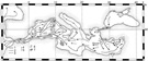General direction of major currents for the zone Mediterranean Sea, Black Sea (without taking into account the seasonal fluctuations).
Issued from Furnestin M.-L., 1979 p.197 in Zoogeography and diversity in plankton. Van der Spoel & Pierrot-Bults (eds). Bunge Sc. Publ., Utrecht.

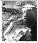Map of the area showing the paths of the main Northern and Balearic Currents and the location of the Rhone River and Ebro River mouths.
Issued from : D. Costalago in Vie Milieu, 2015, 65 (2). [p.102, Fig.1].

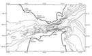Chart of the Strait of Gibraltar with depth contours in meters, based on Defense Mapping Agency (1980) chart No. 52041. Areas deeper than 400 m are shaded.
Overlay. Location of essential topographic features, moorings, transects (solid lines between stars) and way-points (in nautical miles) for the runs.
Issued from : Miller C.B. & Clemons M.J., 1988. - Revised life history analysis for large grazing copepods in the subarctic Pacific Ocean. Progress in Oceanography, 20 (4). [p.41, Fig.2.1].

The tropical-temperate zone of the North-east Atlantic shares 466 species (i.e. 61.3 %) with the Caribbean - Sargasso Sea region and 389 species with the Mediterranean (51.2 %).

Certain species may be considered as relicts from the glacial age: Acartia bifilosa, Chiridius obtusifrons, Paramisophria cluthae, Paraeuchaeta norvegica, Stephos scotti, Lubbockia brevis, Oncaea borealis, O. pumilis , and probably Oncaea englishi. Pseudocalanus elongatus originating in the North Atlantic, and also reported in the Gulf of Guinea, was perhaps introduced by the superficial Gibraltar current. Spinocalanus terranovae, observed recently (Lapernat & Razouls, 2001) in deep water near Malta, was previously only known in the Antarctic as Ctenocalanus citer (Uysal & al., 2002).

For Selifonova & al. (2010) there are 20 mediterranean species that were discovered for the first time for the Black Sea (May-June 2001). Species diversity of Mediterranean copepods was unusually high from the region nearest to the Bosporus. Most probably these invaders were carried by the Lower-Bosporus flow. However, same species were also found in the northwestern Black Sea (in good conditions). Nevertheless, the ballast water commercial ships is a possibility of introduction (for example of invasions of Oithona brevicornis in areas of the ports Novorossiysk, Tuapse, Sevastopol). The marked appearance of 33 Mediterranean copepods taxa in the Western Black Sea confirms that process of Mediterranization of fauna (Pusanov, 1967) is continuing.

401 species are common to the Mediterranean and the Indian Ocean (i.e. 66.2 %).

(For more details on species of the zone Mediterranean - Black Sea (14) see the Chapter (in french) "Distribution géographique des copépodes pélagiques en Méditerranée").

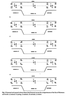Seasonal and annual volume fluxes (km³/season) across the compartments of the Marmara Sea and straits Dardanelles and Bosphorus.
Two-layer flow regimes in the Turkish Strait System introduce the brackisk waters of the Black Sea into the Aegean basin of the northeastern Mediterranean throughout the year. A counter flow carries the salty Mediterranean water into the Black Sea via the Marmara deep basin.
The annual volume influx from the Black Sea to the Marmara upper layer is nearly two-fold the salty water exported from the Marmara to the Black Sea via the Bosphorus underflow.
Issued from : S. Tugrul, S.T. Besiktepe & I. Salihoglu in Mediterranean Marine Science, 2002, Vol. 3/1. [p.37, Fig.3].

Mediterranean Sea and Black Sea

Strait of Gibraltar:
The Strait of Gibraltar, which links the Atlantic and the Mediterranean, is an example of density-driven currents.
The surface inflow of less saline Atlantic water into the more saline Mediterranean gives rise to a deep-water outflow of Mediterranean water into the Atlantic.
The main cause of these water exchanges is the increase in salinity and the difference in sea level produced by the substantial evaporation of Mediterranean waters. According to Nielsen's estimates, the excess of evaporation over freshwater input would remove 3000 cubic kilometres of water per year from the Mediterranean, if Atlantic waters did not enter through the Strait of Gibraltar. The mean levels of the Atlantic and the Mediterranean would show a difference in favour of the Atlantic of a few centimetres, depending on the season, with the level difference varying from year to year.
Aside from the tidal currents that complicate the phenomenon, there is, in the middle of the strait, a permanent surface current flowing from West to East, which varies with the wind and whose average speed exceeds 1 knot, sometimes reaching over 2 knots.
The shape of the shores, both in Spain and North Africa, slightly alters the direction of this current; near the coast, besides the tidal currents, westward-flowing countercurrents occur.
The surface current is felt down to a depth of about 100 m. At greater depth, there is a current flowing in the opposite direction, revealed by salinity measurements. The Atlantic water entering at the surface through the strait has a salinity of 36; at depth, within the strait, the salinity exceeds 37 and even reaches 38, water that can only originate from the Mediterranean.
Idrac, in the narrowest part of the strait, south of Tarifa, observed at the surface a current flowing East-Northeastward with a speed of 1.4 knots; at 100 m, the same direction, speed 0.8 knot; below 100 m the current turns sharply Westward-Southwestward and remains so to the bottom, with a speed of 1.1 knots at 200 m, 4.2 knots at 300 m, 0.9 knot at 400 m, 0.5 knot at 500 m. Other observations have shown that the bottom current was stronger than the surface current, sometimes reaching a speed of 4 knots.
This Mediterranean water, carried at depth through the Strait of Gibraltar, is partly held back by the transverse sills that block the strait, and follows the channels located to the North and South of the Spartel Bank. The deflecting force of the Earth's rotation causes the Mediterranean outflow to preferentially follow the channel on its right (the northern channel), and this Mediterranean water can be traced rounding Cape St. Vincent and then heading Northward along the coast of Portugal. At the same time, however, eddies form on the left of this current, mixing part of the Mediterranean water with Atlantic water, so that, in the end, the Mediterranean water appears to fan out on leaving the strait. Its salinity certainly decreases rapidly, falling to 37 immediately west of the strait, and to 36 at 500 miles. This water of Mediterranean origin, at a depth of about a thousand metres, can be recognised by a slightly higher temperature and salinity than the surrounding layers, as far as the waters off Ireland to the North and the Canaries, even the Sargasso Sea, to the South (G. Roux, 1943).

Western Basin:
Almost everywhere, the influence of the winds predominates in the formation of the currents, which can exceed 2 knots.
The general West-to-East current, which enters at the surface through the Strait of Gibraltar, continues along the Algerian coast at a speed of half a knot in calm weather. Along the coasts of Spain and Morocco, westward-flowing countercurrents are fairly often observed.
The current continues, partly along the western coast of Sardinia, and partly along the northern coast of Sicily, flowing Northwestward along the Italian coasts. In the Gulf of Genoa it turns Westward along the coasts of Provence. In the Gulf of Lion it turns Southward, most often under the effect of strong North to Northwest winds (Mistral and Tramontane) and the bathymetric configuration of the Gulf. The current induced by these gusts can reach speeds of 2 to 4 knots. This general current does not exactly follow the indentations of the shoreline, running directly from one headland to the next, hence the existence, in the bays, of a countercurrent following the shore in the opposite direction to the main current.
Off Marseille, given the configuration of the coast relative to the direction of the North wind, an upwelling mechanism occurs.
Along the Catalan and Spanish coasts, the current flows Southwestward, thus forming a complete counter-clockwise circuit in the western basin of the Mediterranean.
Between Sicily and Tunisia, in the Sicilian-Tunisian Strait, there is an almost permanent eastward current, whose speed can exceed 1 knot.

Eastern Basin:
The general surface current coming from the Alboran Sea follows the Libyan and Egyptian coast Eastward.
Before the regulation of the Nile, brought about by the new Aswan Dam (completed in 1970), during the Nile flood which begins in June-July and ends in September, the eastward current off the delta became irregular; the Nile current was felt 2 to 3 miles from the river mouth, and its fresh waters did not mix with those of the sea. The current resumed its normal direction before reaching Port Said.
Nowadays, the waters of this region have a more normal salinity.
The current flows along the Israeli and Syrian coasts, toward the Northeast and North, at about 6 miles per day.
At the time of the Nile floods, the less saline water was felt along these coasts, where a very marked decrease in salinity was observed in September.
Along the southern coast of Turkey, the current flows Westward. In the Aegean Sea, it flows Northward along the coasts of Anatolia, then, following the Dardanelles current, which flows steadily at a speed of 3 to 4 knots from the Black Sea toward the Mediterranean, the general current turns back Southward through the middle of the Aegean Sea and along the coasts of Greece (which explains why the waters are more saline in the eastern part of the Aegean Sea than in the western part), with an average speed of a quarter of a knot. In the narrow channels, its speed increases, exceeding 1 knot, and can even reach considerable speeds when the wind blows in the same direction as the current (7 knots in the Doro Channel between Andros Island and Euboea).
At Cape Matapan, the current flows Westward; it moves up the Ionian Sea around Greece. Another current follows the coast of Sicily to the South, thus completing the circuit of the eastern basin of the Mediterranean, a counter-clockwise circuit (as in the western basin).

Adriatic Sea:
A general coastal current, arriving through the Corfu Channel, flows Northwestward along the eastern coast, rounds the Gulf of Venice, and flows Southeastward along the Italian coast, thus describing a counter-clockwise circuit.
Off the Lahosta Islands, a branch of this current is deflected Westward and Southwestward, toward Pelagosa and Cape Gargano, where it reinforces the Southeastward current along the Italian coast. Another important branch veers off the Gulf of Kvarner and flows toward the western coast, where it joins the current running Southeastward. The speed of these currents averages 0.3 knot in the southern basin and 0.5 knot in the northern basin; but winds can increase their speed to up to 2 knots.

The Bosphorus and the Dardanelles:
The Bosphorus and the Dardanelles (Hellespont), located at the eastern and western ends of the Sea of Marmara, are traversed by very strong currents. Whatever the prevailing winds, the general current always flows from the Black Sea toward the Sea of Marmara and the Mediterranean. The numerous bends of the channels give rise to countercurrents and eddies.
In the narrowest part of the Bosphorus, off Arnaout Keuy, where the width is only 530 metres, the speed can reach 4 to 5 knots.
In the Dardanelles, the current can reach a speed of 4 knots off Canakkale (Chanak Kalesi).
At depth, the current flows in the opposite direction to the surface current, moving from the Mediterranean and the Sea of Marmara toward the Black Sea. The depth at which the current changes is 15 metres off Istanbul, and 40 metres in the upper Bosphorus. The speed of the deep current can exceed 2 knots. In the upper Bosphorus, north of Sariyer (Therapia), the deep current is normally stronger than the surface current.
The explanation for this double current lies in the density differences between the Black Sea, the Sea of Marmara and the Mediterranean.
The Black Sea has a salinity of 18; it reaches 20 at a depth of 200 metres, and increases slowly toward the bottom without exceeding 22.5. In the Sea of Marmara, the surface salinity is 21, but it increases rapidly with depth, reaching 37.5 at 30 metres and exceeding 38 from 50 metres downward.
The currents of the Bosphorus and the Dardanelles have their speed altered by the direction, strength and duration of the winds. After a prolonged period of North winds, the Bosphorus current reaches its maximum speed, and the surface current extends deeper than usual; with South winds, the speed decreases and sometimes becomes almost nil.

The Black Sea:
The discharge of the great rivers flowing into it, the Danube, Dniester, Dnieper and Don, together with the very abundant atmospheric precipitation, maintain a salinity much lower than that of the Mediterranean and the Sea of Marmara.
The water discharged by the rivers is deflected to the right by the Earth's rotation, and, together with the winds, determines the surface current of the Bosphorus, carrying these waters from the Black Sea toward the Sea of Marmara and beyond toward the Mediterranean.
The accumulation of water toward the Bosphorus is so significant that part of it is pushed back along the coasts of Anatolia, forming an eastward current that follows the contour of the coast. This results in a counter-clockwise circuit, whose speed varies from 0.5 to 1 knot. The current is particularly pronounced between the Danube delta and the Bosphorus, and, with North winds, especially in spring when river inputs are considerable, the speed of this current can exceed 1 knot.
Along the coasts of Turkey and Bulgaria, as far as Balchik Bay, a current opposite to the general current and flowing Northward is observed in the immediate vicinity of the coast. Similarly, along the coasts of Anatolia, between Sinope (Sinop) and Kerempe, there are westward countercurrents.
The waters of the Sea of Azov normally flow at the surface toward the Black Sea through the Kerch Strait (Kerchenskiy Proliv) at a speed close to 1 knot, which can reach 3 knots in spring. After prolonged Northeast gales, which have accelerated the current and lowered the sea level, the current sometimes reverses, flowing then from the Black Sea toward the Sea of Azov, at a speed that can exceed 0.5 knot. This abnormal current is observed mainly in winter.
The Kerch Strait shows that a very shallow depth (7 metres) is enough for double density-driven currents to become established. The water of the Sea of Azov, abundantly fed by the Don River, has a salinity ranging from 7 to 11, whereas the salinity of the Black Sea is 16 to 17.
In the Kerch Strait, a surface current, extending down to a depth of 5 metres, carries the freshened water of the Sea of Azov toward the Black Sea; below it, an opposing current carries the more saline water of the Black Sea into the Sea of Azov.

References:
J. Rouch, 1948. Traité d'Océanographie physique. 3 : Les mouvements de la mer. Payot, Paris.
Contributions to the Oceanography of the Western Alboran Sea. NORDA, 315, April 1985. XXIXth Congress and Plenary Session of the International Commission for the Scientific Exploration of the Mediterranean Sea, Lucerne October 11-19, 1984.
J. Rodriguez, 1982. Oceanografia del Mar Mediterraneo. Edic. Piramide.
P.A. Auger, 2011. - Modélisation des écosystèmes planctoniques pélagiques en Méditerranée nord-occidentale - Impact des eaux du Rhône à l'échelle du plateau du golfe du Lion et variabilité inter-annuelle à décennale au large. Thesis Université Paul Sabatier, Toulouse III, 1-242 pp.
Atlas of Pilot Charts http://msi.nga.mil/NGAPortal/MSI.portal?_nfpb=true&_pageLabel=msi_portal_page_62&pubCode=0003 NATIONAL GEOSPATIAL-INTELLIGENCE AGENCY (USA)

Zones: Venezuela - Caribbean - Sargasso Sea (7) ; NW North Atlantic (Nova Scotia-Labrador Sea) (11)

	7	11
Total species:	714 (27.8 %) (+ 10 ind.)	259 (10.1 %) (+ 2 ind.)
Calanoida:	557	204
other orders	157	55

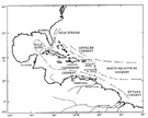Issued from : Murphy S.J., Hurlburt H.E. & O'Brien J.J. in Journal of Geophysical Research, 1999, 104 (C1). [p.1435, Fig.2].
Schematic Caribbean circulation drawn from pilot charts [from Duncan et al.,1982].





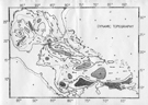Issued from : R. Margalef in The pelagic ecosystem of the Caribbean Sea. Symp. Invest. Res. Caribb. Sea and adjacent region: 1971, 483-498 (UNESCO, SC. 70/D.71/AS). [Fig.1]
Average dynamic topography of the American Mediterranean, in dynamic meters.
For the Gulf of Mexico (North of the double line), data of Duxbury (1962) and contours refered to the surface of 1000 decibars. For the Caribbean (South of the double line), data of Gordon (1967) and reference to the 1200 db level.
The areas of presumible upwelling are covered by points, and the areas of possible sinking are lined.
Arrows indicate the principal currents.

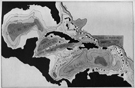Issued from: E. Le Danois in L'Atlantique. Albin Michel (ed.), Paris, 1938. [p.112].
Topography of Caribbean Sea and Gulf of Mexico.





Caribbean Sea and Gulf of Mexico:
The Caribbean Sea and the Gulf of Mexico are crossed by the North Equatorial Current and a fraction of the South Equatorial Current, these two currents having merged west of the region occupied by the equatorial countercurrent, which originates around the 42° West meridian, heading toward the Sierra Leone Basin.
Part of these equatorial currents flows into the Caribbean Sea, through the straits separating the islands, which are often about a thousand metres deep. The westward current is, in all seasons, about 1 knot, sometimes reaching 3 knots in summer. The current skirts the tip of the Yucatan peninsula and enters the Gulf of Mexico. Apart from a slight current that runs all the way around the Gulf of Mexico, the waters head directly for the north coast of Cuba to form the Gulf Stream in the Florida Strait.
The part of the equatorial currents that does not enter the Caribbean Sea runs, at a moderate speed, along the north coasts of Puerto Rico, Haiti and Cuba, and joins the Gulf Stream off the coast of Florida.
In the Caribbean Sea, the current is stronger in the southern part than in the northern part; it rarely exceeds a speed of 2 knots and, strictly speaking, constitutes more of a general water movement than a true current. Along the coasts there are countercurrents whose speed can be fairly high. An eastward countercurrent occurs between the islands bordering the coast of Venezuela and the mainland, but it is mainly off the coast of Colombia that it reaches a speed of 0.5 to 1 knot.
In the southern part off Costa Rica, the countercurrent reaches a speed of 2 knots.
In the Gulf of Honduras, the equatorial current is felt as far as the vicinity of the coast, and it is only close to the shore that a Southward and Eastward countercurrent is observed.
Similarly, along the southern coasts of Cuba and Haiti, there is an eastward countercurrent, whose speed averages 1 knot.
Between Cuba and the Yucatan peninsula, the axis of the northward current lies about 6 miles from the 180-metre depth line of the Campeche Bank, at depths ranging from 360 to 755 metres. The western limit of the current is formed by the Campeche Bank, its eastern limit passing 20 miles from Cape San Antonio (Cuba). From this cape onward, the average current speeds are 1 knot at 30 miles, 1.5 knots at 50 miles, 2.8 knots at 65 miles, 3.5 knots at 78 miles, 0.5 knot at 94 miles, i.e. 20 miles from the Yucatan coast. Along the coast of Cuba and over the Campeche Bank, there is a slight southward countercurrent. The main branch of the equatorial current runs directly from the Yucatan Channel to the Florida Strait at a speed of 2 knots. Another branch of the equatorial current goes around the western Gulf of Mexico at a speed of 1 knot. This branch varies in width over the course of the year, and is felt further offshore from July to October. Throughout the Gulf, near the shore, a countercurrent has a speed of 1 knot in places.
In the centre of the Gulf, around 27° North latitude and 88° West longitude, there is, over a diameter of about 80 miles, a current-free zone where floating plants and debris accumulate, and whose green waters contrast with the blue waters of the equatorial current. As for the Mississippi, its current is felt 10 to 15 miles offshore depending on water levels. The separation between the blue water and the yellow river water is sharply defined.
R. Margalef (1971) compares this American Mediterranean with its European counterpart, both seas presumed to derive from the ancient Tethys. The Mediterranean and the Black Sea have a surface area of 2.996 million km2, compared with 4.319 million km2 for the Caribbean Sea and the Gulf of Mexico. Estimated primary production (g C/m2/yr) is 25-80 for the former, against 40-120 for the latter. It appears that in the second case production is higher than that of its European equivalent, but that its fisheries are under-exploited.
In the first case, exchange with the Atlantic leads to a loss of nutrients, which must be offset by land runoff providing a relatively low, balanced concentration. In the second case, the hydrographic structure and circulation show a much higher phosphate input, the deep basins containing nutrient-rich water; at least at the levels available for fertilisation, the phosphate concentration exceeds 0.3 µg-at. P/l. Water stratification limits the possibilities of vertical mixing, but in certain zones upwellings reach an importance never observed in the European Mediterranean (Sturges, 1965). The Mississippi contributes a significant phosphate input (2 to 19.6 mg P/m3) (Riley, 1937; Davis, 1954), just as the Caribbean islands represent fertilisation sites.
References:
J. Rouch, 1948. Traité d'océanographie physique, p. 309-311. Édit. Payot, Paris.
Atlas of Pilot Charts http://msi.nga.mil/NGAPortal/MSI.portal?_nfpb=true&_pageLabel=msi_portal_page_62&pubCode=0003 NATIONAL GEOSPATIAL-INTELLIGENCE AGENCY (USA)

The Sargasso Sea:
At the centre of the North Atlantic circuit, midway between the Bahamas and the Azores, lies a vast expanse of water known as the Sargasso Sea. Its name comes from the abundance of algae, related to Fucus, which float at the surface thanks to gas-filled bladders that act as floats.
It is rare to find masses of clumped Sargassum exceeding about thirty metres in diameter. Sometimes, under the action of the wind, the Sargassum gathers into long rows; more often it is found in isolated clumps, separated by vast expanses of open water. The abundance of this macroalga varies greatly from year to year; in 1939 J. Rouch observed that the algae were much less numerous than in 1907.
Not only does this abundance of algae make the Sargasso Sea distinct from other parts of the Atlantic Ocean, but its waters also show very marked characteristics.
These waters are not motionless, but animated by various drifts, fairly confused on maps, and take some part in the general circulation. They are notable for their high salinity, above 37, even 37.5, their high temperature, sometimes exceeding 28°C, their dark blue colour, and their great transparency (the Secchi disc is clearly visible to the eye at depths of more than 60 metres). In fact there is no great difference between the waters of the Sargasso Sea and those of the Gulf Stream. The T-S diagrams (temperature and salinity characterising a water mass) for the two regions are often similar. Some have felt it necessary to combine the Sargasso Sea and the Gulf Stream into a single region.
The particular characteristics of this deep sea (its average depth exceeds 4000 m, and depths of nearly 7000 m are found there) are explained by the high salinity resulting from the absence of continental water input, the absence of rain in this zone of tropical calms and intense evaporation, and the currents of saline water surrounding it, a region of low cloud cover and high air temperatures. These saline waters, fairly dense despite their high temperature, tend to sink and carry the surface waters down to depth. Thus, down to more than a thousand metres, temperatures higher than those of neighbouring parts of the Atlantic Ocean are observed in the Sargasso Sea. The transparency of the waters is due to the absence of any terrigenous input, weak circulation, and a greater scarcity of plankton, little stimulated by upwellings of deep water rich in nutrient salts.
It is hardly necessary to recall that this sea is one of the great spawning grounds of eels.
References:
J. Rouch, 1948. Traité d'océanographie physique, p. 309-311. Édit. Payot, Paris.
Neveux J., Vaulot D., Courties C. & Fukai E., 1989. Green photosynthetic bacteria accociated with the deep chlorophyll maximum of the Sargasso Sea. C.R. Acad. Sci. Paris, 308 , ser. III, p. 9-14.
Atlas of Pilot Charts http://msi.nga.mil/NGAPortal/MSI.portal?_nfpb=true&_pageLabel=msi_portal_page_62&pubCode=0003 NATIONAL GEOSPATIAL-INTELLIGENCE AGENCY (USA)

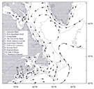Major currents of the northwest Atlantic shelf and Labrador Sea region.
Issued from : E.J.H. Head & D.D. Sameoto in Deep-Sea Res., II, 2007, 54. [p.2688, Fig.1].

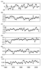Anomalies for the 1960-2003 period for the North Atlantic Oscillation (NAO, A), depth averaged temperatures on the Newfoundland shelf (B), the eastern Scotian shelf (C), and the central/western Scotian shelf (D), and for the depth averaged salinities (E) and stratification indices (F) on the Newfoundland shelf.
Nota: The time series of the NAO index (variations in climate indices) reveals a period of sustained negative values during 1960s and a period of predominantly positive values during the 1990s, the latter also including a dramatic decrease to a negative value in 1996 and subsequent recovery. For 2001-2003, the NAO index was either negative or neutral.
Water temperatures (at station 27) at the east Newfoundland were above normal in the 1960s, coldest in the early 1990s, rose throughout the rest of the 1990s, with 1-year high value in 1996, and did not change much after 1999s. On Misaine Bank on the east Scotian shelf water temperatures were cool in both the early 1960s and the mid-1980s to the early 1990s, with peak values in 1999 and 2000. In Emerald Basin, on the central/western Scotian shelf, water temperatures were low in the 1960s and generally slightly above average in the 1990s, with the 1-year decrease to lower than average values in 1998. On the newfoundland shelf, salinities were generally below the 1960-2003 average after 1990, rising to slightly above average vaues in 2002-2003.
Stratification there generally increased over the 1960-2003, with a slight decrease in 2002-2003.
The relationship between temperature and the NAO index was examined using lags of up to 4 years for the three ares. The 1960-2003 depth averaged water temperatures were negatively correlated with the NAO index on the Newfoundland shelf with no lag, negatively correlated with the NAO index on the eastern Scotian shelf with a 2-year lag, and posiitively correlated with the NAO index on the western Scotian shelf with a 2-year lag.
Issued from : E.J.H. Head & D.D. Sameoto in Deep-Sea Research II, 2007, 54. [p.2691, Fig.3].

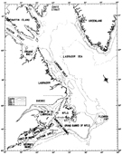Study areas of the northwest Atlantic for which planktonic copepod species occurrences were recorded.
Issued from : M.J. Tremblay & J.T. Anderson in Annotated species list of marine planktonic copepods occurring on the shelf and upper slope of the northwest Atlantic (Gulf of Maine to Ungava Bay). Can. Spec. Publ. Fish. Aquat. Sci., 69. [p.2, Fig.1].
This reproduction is a copy of an official work that is published by the Government of Canada and it has not been produced in affiliation with, or with the endorsement of the Government of Canada.

Currents of the Gulf of St. Lawrence.
Issued from : Published by Oceans and Science Branch, Fisheries and Oceans Canada in The Gulf of St. Lawrence. A unique Ecosystem, 2005.
This reproduction is a copy of an official work that is published by the Government of Canada and it has not been produced in affiliation with, or with the endorsement of the Government of Canada.

The Gulf Stream:
It results from the North Equatorial and South Equatorial currents, both flowing from the East (African continent) toward the West (American continent), originating in the trade winds blowing from Northeast to Southwest in the boreal hemisphere and from Southeast to Northwest in the austral hemisphere.
These trade winds drive the waters in such a way that the equator is flanked by a surface North Equatorial Current and a South Equatorial Current, both flowing from East to West.
Of these two currents, the stronger is the southern one. It originates near Annobón Island, or immediately south of the equator between longitudes 2° and 8° East, and is felt over a wide band extending from 2°N to 3°N down to latitude 20° South. It begins its course at a speed of about 15 miles per day. Its direction gradually turns Northward, its speed increasing progressively, especially west of the Greenwich meridian; it is stronger during the Northern Hemisphere summer, and reaches a speed of 2.5 knots near the coast of Brazil. Off Cape San Roque, the current splits, the main branch following the coast of Guiana and joining the North Equatorial Current, which it reinforces, while the other branch bends Southward.
The North Equatorial Current originates off the Cape Verde Islands; its direction is only well defined between latitudes 5° N and 10° N. Its speed is generally weaker than that of the South Equatorial Current. However, during summer, around the 20th degree of West longitude, speeds of nearly 3 knots have been observed. These flows enter the Caribbean Sea and the Gulf of Mexico through the Yucatan Channel.
It is thus an enormous quantity of warm water that enters the Gulf of Mexico and eventually emerges as a powerful jet through the strait between the Florida Keys and Cuba, a location considered to be the origin of the Gulf Stream. Average speeds of 3 to 5 knots are at their maximum off Cape Florida (also called the "Florida Current"). In 1948, Jean Rouch estimated its volume at 24 million cubic metres per second, or 22 times more than all the rivers on Earth combined. Its temperature is 27°C and its speed about ten kilometres per hour. In this part of the Gulf Stream, surface waters have a salinity of 36 to 36.5 at a depth of 200 metres, and the average surface water temperature is 26.5°C. From this point onward, the Gulf Stream fans out Northeastward under the combined effect of the changing direction of the shoreline and the Earth's rotation. At the same time, it gradually slows down, its speed averaging 2 knots off Savannah, and 1.5 knots off Cape Hatteras; however, a marked annual variation in current speed is observed, being twice as strong from February to April as from August to October. Around latitude 30° N, the Gulf Stream receives the inflow of waters from the Antilles Current, the two currents sometimes being separated from one another, up to this latitude, by a slight southward countercurrent. Measurements have shown that the Northeastward current is no more than 130 miles wide at the surface; at depth, the current is detectable beyond 1000 metres, and down to 500 metres it often has a speed of more than 1 knot. On its course from the tropics toward higher latitudes, its temperature drops by barely one degree for a 10° change in latitude. Down to 500 metres depth, the Gulf Stream waters are noticeably warmer and more saline than the surrounding waters. It is deflected away from the United States, from Cape Hatteras onward, by the effect of the Earth's rotation and the flow of the cold Labrador Current, coming from the Baffin Sea, near the Grand Banks of Newfoundland. These cold, relatively low-salinity waters sink beneath those of the Gulf Stream. Mixing of the waters eventually occurs; the temperature of the Gulf Stream decreases noticeably, barely exceeding 20°C at the surface, and falling below 15°C at depths of 200 to 300 metres; its salinity does not exceed 36.5 and there is no longer any increase in salinity with depth, as was the case in the Florida Current and near Cape Hatteras.
While the characteristics of the Gulf Stream are clearly defined between the Florida Strait and southern Newfoundland, they no longer hold once it meets the Labrador Current. The impetus it received in the Florida Strait is partly spent after a long course of 1800 miles. The high temperatures, strong salinity and high speed that characterised it have gradually diminished, along with its fine blue colour. But the water it carries continues to drift Eastward and Northeastward. The drift due to the prevailing westerly winds adds to this, but this drift does not play the predominant role, since, as a result of the Earth's rotation, the current bends Southeastward, while the sinking of the much colder and denser Arctic polar waters maintains what is now called the North Atlantic Drift, which continues along the coasts of Norway, reaching the Murman coast, where the ports of Hammerfest, beyond the Arctic Circle, and Petsamo remain ice-free year-round. Its influence ends at Spitsbergen.
References:
J. Rouch, 1948. Traité d'océanographie physique, p. 309-311. Édit. Payot, Paris.
Atlas of Pilot Charts http://msi.nga.mil/NGAPortal/MSI.portal?_nfpb=true&_pageLabel=msi_portal_page_62&pubCode=0003 NATIONAL GEOSPATIAL-INTELLIGENCE AGENCY (USA)

 

Zones: North-Eastern North Atlantic (9) ; North Sea-Baltic Sea (9') ; North Atlantic (Southern Iceland) (10)

	9	9'	10
Total species:	389 (15.1 %) (+ 4 ind.)	114 (4.2 %) (1 ind.)	203 (7.9 %) (0 ind.)
Calanoida:	293		186
other orders	96		17

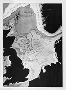Topography of the North Sea.
Issued from: E. Le Danois in L'Atlantique. Albin Michel (ed.), Paris, 1938 .[p.80].

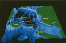Feeding areas of herring (after Dragesund & al., 1997), blue whiting (after Blindheim & Skoldal, 1992), and mackerel (suggestive) in the Norwegian Sea.
Issued from : S. Kaartvedt in ICES Journal of Marine Science, 2000, 57 (6). [p.1821, Fig.1].
Herring (Clupea harenus) enter the feeding area from spawning grounds on the Norwegian Shelf, expanding westwards and northwards in accord with the progression of the subsequent spring production in those areas.
Blue whiting and mackerel migrate eastwards and northwards from the spawning grounds west and south of the United Kingdom.
Note the bathymetric map by Bjørn Gjevik, University of Oslo.

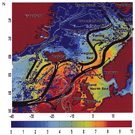Schematic of the major pathways of near-surface Atlantic water in the northern North Atlantic and Nordic Seas (dark arrows) as derived from near-surface Lagrangian drifter data, in context of superimposed sea surface temperature from AVHHR image in March, 1991.
Issued from : K.A. Orvik in Geophysical Research Letters, 2002, 29 (19). [p.2.2,Fig.1].

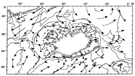Main currents around Iceland.
Issued from : D.J. Beare, A. Gislason, O.S. Asthorsson & E. McKenzie in ICES J. Mar. Sci., 2000, 57 (6). [p.1546, Fig.1].
Atlantic Water (flighted arrows); Polar Water (normal arrows): Arctic Water; Coastal Water (thin broken arrows).

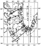The current systems (after Hansen & Killerich) and the location of the hydrobiological sections.
Issued from : E.A. Pavshtiks in Sarsia, 1968, 34. [p.384, Fig.1].
1 - Canadian Polar and East-Greenland Currents. 2 - Irminger Current. 6 - Circulation of subarctic waters. 4 - West-Greenland Current. 5 - Standard sections of PINRO. 6 - Standard sections during Norwestland I and III. 7 - April-July. 8 - August-September.
7 and 8. Sampling stations.
Davis Strait is here defined as that area between Greenland and Canada bordered by latitudes 55° and 67° N.
Hydrological conditions in the Davis Strait are very similar to those in the Norwegian, Greenland, Barents and Karak Seas though the Davis Strait differs in its greater proximity to the Atlantic Ocean. Arctic and Atlantic waters meet and mix in the Davis Strait, thus forming ''the secondary polar front'' and a cimplex system of circulation of subarctic waters. This creates special conditions which affect the development of the plankton. The influence of Atlantic and Arctic waters upon composition of zooplankton in the Davis Strait has been studied by Aurivillius, 1896; Jespersen, 1934; Kielhorn, 1952; Gruzov, 1961; Kramp, 1963; Grainger, 1961, 1963; Pavshtiks, 1964; Semenova, 1964.

 

Zones: Antarctic (4) - Sub-Antarctic (3) ; Arctic Ocean (27)

	4 or 3	27
Total species:	394 (15.4 %)(+ 11 ind.)	184 (7.2 %) (+ 7 ind.)
Calanoida:	331	147
other orders	63	37

Antarctic and Sub-Antarctic species

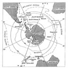A total of 394 species, i.e. 14.6 % of the marine species, have been reported in the Antarctic Ocean (continent and southern parts of the three oceans). 274 species are present in the South Pacific, 223 species in the southern Indian Ocean and 223 species in the South Atlantic, and some are found in the southern parts of all three oceans. One hundred and fourteen found in contact with the continent or near the ice pack correspond to species adapted to the coldest temperatures.

In view of the imprecisely defined latitudinal limits for the Antarctic convergence, it is probable that two hundred and twenty three forms (i.e. 83.2 %) observed in the sub-Antarctic province come from sub-tropical and temperate zones, carried by surface or deep-water currents. This relatively high immigration level for Copepoda is perhaps accidental, and may constitute pseudopopulations as noted for coccolithophores by Winter et al. (1999) in the Weddell Sea.

Longhurst (1998, p.341) situates this sub-Antarctic ring between the limits of the Polar Front to the South and the sub-Antarctic Front at its sub-tropical convergence to the North.

Fourteen species are characteristic of the sub-Antarctic region, although it is difficult to define the latter from hydrological (Gamberoni et al., 1982) or current (Y. H. Park, 1999) data: Acartia ensifera, Aetideus pseudarmatus, Euchirella latirostris, E. similis, Calanoides macrocarinatus, C. patagoniensis, Candacia cheirura, Clausocalanus ingens, Drepanopus forcipatus, D. pectinatus, Paraeuchaeta eltaninae, Lucicutia rara, Calocalanus fiolenti, C. longispinus.

Thirty four species have been reported only on one side or the other of the Antarctic convergence (or Polar Front): Aetideopsis tumorosa, Aetideus australis, E. rostromagna, Pseudochirella hirsuta, P. mawsoni, Euaugaptilus aliquantus, E. parasetosus, Haloptilus ocellatus, Calanus propinquus, C. simillimus, C. maxima, Clausocalanus brevipes, C. laticeps, Ctenocalanus citer, Subeucalanus longiceps, Paraeuchaeta antarctica, P. biloba, P. dactylifera, Paraeuchaeta parvula, P. rasa, P. regalis, Heterorhabdus austrinus, H. farrani, H. pustulifer, Bathycalanus eltaninae, B. inflatus, Bradycalanus pseudotypicus, Metridia gerlachei, Cornucalanus robustus, Amallothrix dentipes, Stephos longipes, Oithona frigida, Oncaea curvata, Triconia antarctica.

A detailed analysis of the distribution of species is provided by Razouls et al. in Workshop Evolutionary Biology of Antarctic organisms. Curitiba , Brazil . 12-15 May, 1999.

Recent revision by Park & Ferrari, 2009.

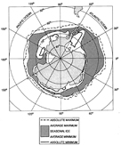Antarctic Ocean showing the average and absolute maximum and minimum seasonal ice cover (modified from Maykut, 1985).
Issued from : R.J. Conover & M. Huntley in J. Mar. Syst., 1991, 2. [p.2, Fig.1]

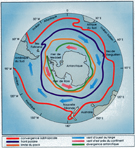Southern Ocean.
Issued from : P. Tréguer & G. Jacques in La Recherche, Vol. 17, 1986, n°178. [p.748, Fig.2]

The Southern Ocean occupies 20% of the oceans. It takes the form of a ring 76 million km² bounded on the north by the Subtropical Convergence and south by the Antarctic continent. By convention we distinguish the Southern Ocean to the Antarctic Ocean, located him south of the polar front. This ocean is covered by ice with a maximum extension in winter reached 25 million km² (limit of pack).
Ocean-atmosphere interactions and the wind regime (easterly winds near the continent and winds west off) are the source of surface areas of discontinuities such as antactic divergence where the deep waters are rich in nutrients, rising from 2 to 3000 m to the surface. Instead, the convergence zones (Antarctic Convergence or Polar Front and Subtropical convergence) are associated with cold-water dives.

Wind and water transitions in the Southern Ocean.
Issued from : G.E.R. Deacon in Deep-Sea Res., 1982, 29 (1A). [p.2, Fig.1]

Nota :
The Antarctic divergence is the transition region between the east and west winds. The dotted line nearest the continent shows the location of the average wind boundary. It happens in 68 to 69°S in the Weddell Sea, in 62 to 63°S where the continent extends farther north in the Indian Ocean sector, and in 70 to 71°S north of the Ross Sea. It should be accompanied by evidence of upwelling, and the full line close by shows the circumpolar salitity maximum at 200 m (plotted by Gordon & al., 1978). The only serious discrepancy occurs north of the Ross Sea where other factors may be involved.
The Antarctic convergence : The second dotted line shows the calculated position of the strongest average west wind and maximum northward Rkman drift, and the full line near it is the Antarctic convergence. Although the closely spaced observations and satellite imagery available today emphasize its variability, they are relatively minor variations about what, in the middle of such a wide ocean, must be regarded as a remarkably predictable frontal zone where cold Antarctic water slips below and mixes with warmer water (Kort, 1967). At the surface it is marked by steepening of the meridional gradients of temperature, silicate, and other nutrients, by transitions in phytoplankton and zooplankton, and by a noticeable difference in climate. There is much eddying and interleaving of cold and warm water, but the sustained presence of a weak temperature minimum below the warmer water north of the front is a clear indication of continued sinking. The position of the convergence is based on the finding by Deacon (1933) and MacKintosch (1946) that the surface discontinuity generally occurs close to the latitude where the temperature minimum characteristic of the Antarctic water dips below 200 m on its relatively steep descent below the warmer water. Temperature profiles farther south are clearly marked by a temperature minimum at 100 to 150 m between warmer, less saline, surface water and warmer, more saline, deep water. Profiles farther north are just as clearly marked by warmer, generally well-mixed, water extending well below 200 m. There is greater variability, and more difficulty in interpolating between contra-indicating data, near the S-shaped bend of the convergence in the Scotia Sea. The early studies (Deacon, 1933 ; MacKintosh, 1946) recognized some irregularity and variability in the position of the front.
Although the circumpolar current must be primarily wind driven, its course must be also depend on other factors, for instances the bottom topography, the S-shaped bend of the convergence in the Scotia Sea seems likely to be due to the northern arm of the Scotia ridge.
The effects of heatinh, cooling, and water exchanges on the density distribution and the patch of the current are not so readily apparent, but Stommel (1980) shows how they may determine the latitude in which the main volume of water sinks to form the Antarctic Intermediate Current.
The subtropical convergence : The northernmost full line shows the position of the subtropical convergence, a sharp transition between subantractic water and warmer, more saline water partly derived from strong southward currents. It is generally marked by a surface-temperature discontinuity of 4 or 5°C and a salinity difference of 0.5 p.1000. A particularly sharp crossing was noticed in 41°S southeast of Cape Town (see Würst, 1926). The dotted line close by in figure 1 shows where the calculated Ekman drift, decreasing rapidly to the north, is most convergent. The data compiled over many years usually allow it to be located to within 1 or 2 degrees of latitude, and there are sufficient observations to fix its position in the middle of the Atlantic, Indian, and Pacific sectors. There are special conditions south of the Brazil, Agulhas, and East Australian currents where patches of warm water separate off from the main currents. South of the Brazil current, for example, the main boundary between subtropical and subantarctic waters occurs near 42 to 43°S but the historical data show that patches of the more saline water have reached 47 to 48°S. There is also much irregularity at the boundary with the Falkland current between the Brazil current and Patagonia.

Temperature section and Salinity in the Indian Southern Ocean along 66°30'E between 40 and 62°S in March 1977.
Issued from : L. Gamberoni, J. Geronimi, P.F. Jeannin & J.F. Murail in Oceanologica, 1982, 6 (3). [p.291, Figures 2, 3]

The data show a frontal zone between 43 and 46°S which separates the antarctic and subtropical regions and within which is concentrated most of the circumpolar current. The frontal zone is due to the coalescence of the antarctic and subtropical convergences into a single convergence zone, effectively eliminating the subantarctic region.
The frontal zone which is located between 43 and 46°S in the Kerguelen region (60-75°E) is located 3 degrees further north, between 41 and 43°S, in the Crozet region (50°E).
The coalescence of the two fronts was due to the northward translation of the antarctic convergence west of Crozet Islands, a possible effect of the bottom topography.

Oxygen section in the Indian Southern Ocean along 66°30'E between 40 and 62°S in March 1977.
Issued from : L. Gamberoni, J. Geronimi, P.F. Jeannin & J.F. Murail in Oceanologica, 1982, 6 (3). [p.292, Figure 4]

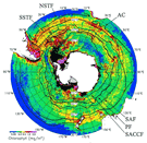Mean SeaWiFS chlorophyll concentration during austral summer (December 1997 through February 1998) and mean location of the major SO fronts. Displayed fronts include the PF [from Moore et al., 1999a], the SACCF, the SAF [from Orsi et al., 1995], the NSTF and SSTF, and the AC [from Belkin, 1993, 1988; Belkin and Gordon, 1996].
Issued from : Moore, J.K., Abbott, M.R., 2000. - Phytoplankton chlorophyll distributions and primary production in the Southern Ocean. Journal of Geophysical Research, 105(C12) : 709-722. [p.711, Fig.3]

   Abbreviations :

SACCF :	Southern Antarctic Circumpolar Current Front
PF :	Antarctic Polar Front (Antarctic Convergence)
SAF :	Subantarctic Front
SSTF :	South Subtropical Front
NSTF :	North Subtropical Front
AC :	Aghulas Current

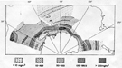The distribution of zooplankton biomass in the Southern Ocean in the 100-0 m layer (mg/m3) in January-May 1956 and 1957.
Issued from : N.M. Voronina in Sarsia, 1968, 34. [p.282, Fig.4]

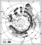Map of zooplankton biomass of the Southern Ocean in the 100-0 m layer.
Issued from : N.M. Voronina & A.G. Naumov in Oceanology, 1968, 8 (6). [p.837, Fig.2]

1: < 10 mg/m³; 2: 10-49 mg/m³; 3: 50-99 mg/m³; 4: >100 mg/m³.

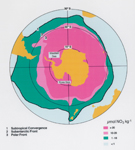Antarctic chart of fronts and nitrate concentrations (Claude Razouls pers. comm.)

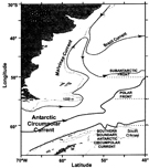Chart of fronts and general pattern of the Southwestern Atlantic Ocean during January 2001.
Issued from : G.A. Thompson, E.G. Dinofrio & A. Alder in J. Plankton Res., 2013, 35 (3), Fig.1

Nota: Structure, abundance and biomass size spectra of copepods and other zooplankton communities in upper waters of the Southwestern Atlantic from 37-61°S, 44-56°W.

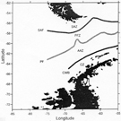The fronts and zones in the Drake Passage.
Issued from :T.J. Grose, J.A. Johnson & G.R. Bigg in Deep-Sea Res. I, 1995, 42 (3). [Fig.1].

Subantarctic Zone (SAZ), Subantarctic Front (SAF), Polar Frontal Zone (PFZ), Polar Front (PF), Antarctic Zone (AAZ), Continental Water Boundary (CWB) and Continental Zone (CZ).

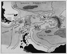Topography of the South Atlantic (sub and antarctic regions).
Issued from: E. Le Danois in L'Atlantique. Albin Michel (ed.), Paris, 1938 . [p.112].

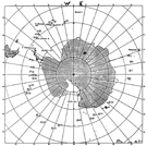The position of the biological stations of «Norvegia» 1930-1931.
Issued from : P. Ottestad in Scient. Results Norw. Antarct. Exped., 1936, 15. [p.7, Fig.1].

The research vessel «Norvegia», on the 14th October passed Bouvet Island and proceeded thence to the Eastward, past Kerguelen, through the Ross Sea, Bellinghausen Sea and the Weddell Sea. In March 1931 she went back to Bouvet.
The expedition's stations were spread over a very great area and were taken at very different periods of the Antarctic summer. The first stations, east of Kerguelen, were taken in the latter half of November, the last in the weddell Sea in the latter half of January. The hydrographical conditions at one and the same place will naturally have changed very much during the course of such a long period. It is, however, of the very greatest importance to be able to determine whether a station has been taken in an Antarctic or sub-Antarctic area? The border-line between these areas of sea, the Antarctic convergence or polar front, is variously situated in the various areas of the Antarctic Ocean. According to Sverdrup (1933) it lies in the Atlantic and Indian Ocean at about 50°S, whereas, in Bellinhausen Sea it runs at about 60°S.

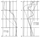The variation of the temperature with depth at stations 5, 7, and 13 (figure left side) and 19, 20, 22, and 24 (figure right side).
Issued from : P. Ottestad in Scient. Results Norw. Antarct. Exped., 1936, 15. [p.9, Figs. 2, 3].

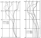The variation of the temperature with depth at stations 27, 28, 34 , and 38 (figure left side) and 41, 42, 46, and 48 (figure right side).
Issued from : P. Ottestad in Scient. Results Norw. Antarct. Exped., 1936, 15. [p.10, Figs. 4, 5].

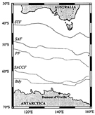Map of the average positions of the fronts in the Indian sector of the Southern Ocean (south of Australia) during the austral summer (December-February) after Orsi & al. (1995).
Issued from : K.T. Takahashi, G.W. Hosie, D.J. McLeod & J.A. Kitchener in Polar Science, 2011, 5. [p.136, Fig.1 (modified)].

STF: Sub-Tropical Front; SAF: Sub-Antarctic Front; PF: Polar Front; SACCF: Southern ACC Front; Bdy: southern boundary of the ACC.
ACC = Antarctic Circumpolar Current.
The southern (SAF-S) branch of the SAF was located at 51°S-53°S. The northern (PF-N) branch of the PF was typically located at approximately 54°S but can be evident at 56.5°S. The PF-S was identified around 60°S. The region north of the SAF-S is defined as the Inter Sub-Antarctic Front Zone (ISAFZ), the region between the SAF-S and the PF-N as the Polar Frontal Zone (PFZ), the region between the two branches of the PF as the Inter Polar Frontal Zone (IPFZ) and the region to the south of PF-S as the Antarctic Zone (AZ).

Antarctic waters patches near of bottom (after Wüst, 1936).
Issued from : J. Rouch in Traité d'océanographie physique. 3 Les mouvements de la mer. Édit. Payot, Paris, 1948. [p.381, Fig.174].

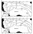Sampling sites and ACC (Antarctic Circumpolar Current) front configuration during sampling.
A) 30th Cruise of R/V "Akademik Ioffe" (during the Southern Hemisphere Summer, December 2009–January 2010).
B) 31th Cruise of R/V "Akademik Sergey Vavilov" (during the Antarctic Spring, October–November 2010).
STF: the Subtropical Front, SAF: the Subantarctic Front, PF: the Polar Front, SACCF: the Southern ACC Front, STZ: the Subtropical Zone, SAZ: the Subantarctic Zone, PFZ: the Polar Front Zone, AZ: the Antarctic Zone.
Issued from : A.N. Stupnikova et al. in Journal of Marine Systems, 2013. 128 [p.176, Fig.1].

Antarctic Ocean:
Driven by the westerly winds, which blow fairly steadily across the latitudes between the 40th and 60th parallels, the surface waters of the Southern Ocean are set in motion by a vast eastward drift, whose speed can exceed 1 knot.
The northern limit of this drift is fairly well marked by the subtropical convergence line, and its southern limit by the Antarctic or sub-polar convergence line. This Antarctic convergence line coincides with the location of the points showing a maximum surface density. Between the temperate latitudes and the Atlantic there is a region where the density of seawater reaches a maximum value, of the order of 1.02725. To the North and South of this region, situated approximately around the 60th degree of latitude, the density decreases, reaching 1.02650, and even 1.026, near the Antarctic continent, and even lower values, close to 1.02550, near Tierra del Fuego, the Cape of Good Hope and Tasmania.
South of this line, around the Antarctic continent, the currents have a northward component, often very clearly marked. The icebergs and ice encountered as far as lower latitudes are evidence of this northward drift. These northward currents have been the subject of direct observations. At the edge of the pack ice, J. Rouch observed, aboard the Pourquoi-Pas?, a fairly strong current, despite a very strong Northeast wind; this current was violent enough to undermine the pack ice from below, thus creating open-water clearings.
In the Weddell Sea, the existence of this current was clearly demonstrated by the drifts of the Deutschland and the Endurance.
The Deutschland, trapped by ice on 6 March 1912 at 74° South latitude and 30° West longitude, drifted first Northwestward, then Northward, and was freed on 23 December 1912 at 64° latitude, having covered 600 miles in 9 months and 17 days, at an average speed of 2 miles per day.
The Endurance, trapped in the ice at 77° South latitude on 5 May 1915, was wrecked on 27 October at 69° latitude, after covering 480 miles in 172 days, at an average speed of 2.8 miles per day. The survivors, taking refuge on an ice floe, continued to drift as far as the 63rd parallel.
The influence of this northward drift is evident in sea water temperatures; whereas west of Graham Land the zero-degree sea water isotherm broadly follows the direction of the shoreline and bends as far as the 69th, even the 70th degree in the Bellingshausen Sea, the same isotherm does not extend south of the 60° parallel in the Weddell Sea sector, and further East rises back to the 54th parallel.
Likewise, the 5° isotherm, which west of the Cape Horn meridian broadly follows the 58th parallel, rises to the 55th degree under the meridian of the Falklands, is found at the 52nd degree under the meridian of South Georgia, and at the 48th degree under the Greenwich meridian.
This northward current propagates toward lower latitudes (the Falklands Current), bringing to the vicinity of the Falkland Islands often considerable quantities of icebergs, which can reach the latitude of Montevideo.
In the Ross Sea, there is also a northward drift, but less pronounced than in the Weddell Sea. The Aurora, trapped in the ice in May 1915 at 78° latitude, eventually reached open sea north of Victoria Land after a 9-month drift.
South of the polar circle, the winds blow mainly from the East, and under their influence the surface sea currents have a westward component, where the shape of the coastline does not prevent it.
Deep circulation has been studied during polar expeditions, in particular by the Discovery I & II (see G.E.R. Deacon, in Discovery Reports, XV, 1937). There are two Antarctic convergence lines in the southern seas; one line lies roughly between 50° and 55° latitude. The 5°C isotherm broadly traces its path. It is from this line that the surface layer sinks beneath the subtropical waters. Near the convergence line, a current of Antarctic water originates, drifting Northward while sinking to depths of about 900 metres. This is fairly cold water, with a high oxygen content, but distinguished chiefly by a lower salinity than that of the layers above and below it. This water is known as Antarctic or sub-Antarctic water.
At a greater depth, between 1000 and 3000 metres, an inflow of relatively warm, saline water coming from the North gradually approaches the surface, and is distinguished by a relative temperature maximum (the deep northern current).
Finally, at even greater depths, exceeding 3000 metres, relatively saline waters are found, but with a very low potential temperature (bottom current). This current has significant northward branches, and travels all the way around the Antarctic continent from West to East. It appears to originate in the Weddell Sea. It is in this deep sea that the inflow of relatively warm Atlantic waters extends furthest South, as far as the 78th degree of latitude. There they lose their heat, contributing to the melting of the ice, become very cold while remaining fairly saline, and sink to the bottom. The Ross Sea, much shallower than the Weddell Sea, does not appear to play any direct role in this deep circulation.
References:
J. Rouch, 1948. Traité d'océanographie physique. 3, Édit. Payot, Paris
Atlas of Pilot Charts http://msi.nga.mil/NGAPortal/MSI.portal?_nfpb=true&_pageLabel=msi_portal_page_62&pubCode=0003 NATIONAL GEOSPATIAL-INTELLIGENCE AGENCY (USA)

Arctic and sub-Arctic species

407 species (of which 9 are questionable), i.e. 16.7 % of the marine species, have been reported in the Arctic and its surrounding seas (zones 10, 23, 24, and part of 9)

191 species are restricted to the Arctic polar basin (zone 27) (incl. ind.), of which 50 are endemic (incl. 7 ind.).

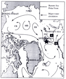Issued from : R.C. Sundt & W. Melle in Mar. Ecol. Prog. Ser., 1998. [p.208, Fig.1]

Major circulation in the Atlantic and Arctic Oceans (after Grotefent & al., 1998); coastlines from GMT (Generic Mapping Tools), Wessel & Smith, 1995.
(black star) Present observation of Calanus marshallae; (white star) observations from Frost, 1974.
CB: Canadian Basin; MB: Makarov Basin; EB: Eurasian Basin; ESC: East Spitsbergen Current; SPG: Subpolar Gyre. Rectangles A and B denote sampling areas for stations.

Map of the northern Bering Sea and Chukchi.
The box marks the survey area of the hydrographic conditions (temperature, salinity and chlorophyll) and Gray whale counts during June to September. The arrows show the prevailing current regime.
Issued from : B.A. Bluhm, K.O. Coyle, B. Konar & R. Highsmith in Deep-Sea Resaeach, 2007, 54. [p.2921, Fig.1]. .

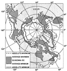Arctic Ocean showing the average and absolute maximum and minimum seasonal ice cover (modified from Maykut, 1985).
Issued from : R.J. Conover & M. Huntley in J. Mar. Syst., 1991, 2. [p.2, Fig.1]








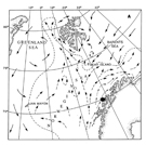The Barents Sea and part of the North Atlantic.
Issued from : F. Norrbin in Dissertation, Unv. Göteborg, Fac. Nat. Sci., 1992. [p.7]

Arrows show the major surface currents; dashed arrows represent warm currents and whole arrows cold currents.
The large, solid arrow points at Tromsø (Northern Norway).



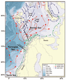A schematic representation of the main currents and topography in the Barents Sea.
Issued from : P. Dalpadado, R.B. Ingvaldsen, L.C. Stige, B. Bogstad, T. Knutsen, G. Ottersen & B. Ellertsen in ICES Journal of Marine Science, 2012, 9. [Fig.1]

The location of the two standard sections; the FB section at the western entrance to the Barents Sea, and the Gimsøy section in the Norwegian Sea, is indicated.





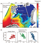Climate effects on Barents Sea ecosystem dynamics.
Issued from : P. Dalpadado, R.B. Ingvaldsen, L.C. Stige, B. Bogstad, T. Knutsen, G. Ottersen & B. Ellertsen in ICES Journal of Marine Science, 2012, 9. [Fig.2]

(a) Mean temperature, 50-200 m, August to early October, based on observations from 1970 to 2010.
The water masses are defined as the Atlantic water (AW: T > 3°C), arctic waters (ArW = T < 0°C), and mixed waters (0°C < T < 3°C).
The grey outline shows the domain for which the area and mean temperatures calculations are performed. The standard FB section is indicated by a black line.
(b) Regression analyses between the areas of AW, ArW, and mixed waters and mean temperature in the three water masses.

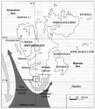Schematic map of sea currents influencing South and West Spitsbergen (light-grey : Arctic Water ; dark-grey : Atlantic Water).
Issued from : L. Stempniewicz, K. Blachowiak-Samolyk & J.M. Weslawski in Deep-Sea Research, 2007, 54. [p. 2940, Fig .2].

Nota : Climate variability in the polar regions in the North Atlantic and vicinity, both near-decadal (e.g. related by the North Atlantic Oscillation or NAO) and longer-terms, leads to changes in large-scale circulation patterns and the hydrologic regime of the northern North Atlantic (see Hurrell, 2003). A crucial oceanographic consequence of a positive NAO index is an increase in the flow of warm Atlantic water into Arctic Ocean (see Dickson & al., 2000). This in turn influences the distribution, abundance, composition and size structure of zooplankton communities (see Beaugrand & al., 2002a). Changes in the size and energy content of key zooplankton prey affect energy transfer in the pelagic food-web. Along with the increased influx of Atlantic waters, Arctic zooplankton communities dominated by large coldwater species, retreat to be replaced with small plankters associated with warmer waters during a positive NAO (see Beaugrand & al., 2002b). Such shifts in zooplankton communities have important consequences for the animal specie that tap into this food base (see Weslawski & al., 1999 a, 2000 ; Karnovsky & al., 2003). Because of differences of the feeding between birds and fish, domination of large crustaceans in zooplankton favours the feeding of plankton-eating seabirds, while the dominance of small forms redirects the food chain to plankton-eating fish, and only then to fish-eating birds (Guillemots for example). Thus, plankton-eating birds should dominate Arctic avifauna in cold periods and recess in warmer periods, when fish-eaters dominate (see Kitaysky & Golubova, 2000). Southern and western Spitsbergen are influenced by different ocean currents (Figure 2). The Sørkapp Current brings cold, arctic waters from northeast with a zooplankton community represented by Calanus glacialis, while the warm water West and South Spitsbergen Currents (branches of the North Atlantic Current that itself is an extension of the Gulf Stream) carry small calanoids, Calanus finmarchicus predominates. The extension of each current and hence proportions of arctic and Atlantic water massesaround South Spitsbergen varies depending on the NAO phase. Total zooplankton biomass is similar in the two water masses, however, the deficiency of large (> 3 mm) crustaceans in Atlantic water dramatically decreases the feeding efficiency of planktivorous seabirds.

Schematic of the major pathways of near-surface Atlantic water in the northern North Atlantic and Nordic Seas (dark arrows) as derived from near-surface Lagrangian drifter data, in context of superimposed sea surface temperature from AVHHR image in March, 1991.
Issued from : K.A. Orvik in Geophysical Research Letters, 2002, 29 (19). [p.2.2,Fig.1].





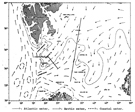Issued from : A. Hassel in Zooplankton investigations near ice edge in the western Barents Sea. Havforskningsinstitutttet, Rapport/Notat Nr. BKO 8308. Biol. og kjem. oceanografi, 1983. [Fig.5].

Schematic picture of the currents and the Polar front (long dotted line) in the Barents Sea. Straight lines indicate the studied sections. (After Loeng, 1983).



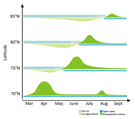Issued from : E. Leu, J.E. Søreide, D.O. Hessen, S. Falk-Petersen & J. Berge in Progress in Oceanography, 2011, 90. [p.19, Fig.1].

Conceptual overview of the primary production regimes in the European Arctic along a latitudinal gradient. Modified after Zenkevitch (1963) and Falk-Petersen & al. (2007).





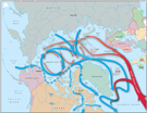Movement of water in the Arctic Ocean.
Blue arrows show cold, relatively fresh water and red arrows show warm, salty water.
Illustration by Jack Cook, WHOI (Woods Hole Oceanographic Institute).






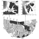Issued from : M. Daase, S. Falk-Petersen, Ø. Varpe, et al. in Can. J. Fish. Aquat. Sci., 2013, 70. [p.873, Fig.1].

Amundsen Gulf, Franklin Bay, Kongsfjorden, and Rijpfjorden. Also marked are North Water Polynya, Disko Bay, Lurefjorden, and the White Sea.






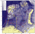Issued from :E. Eriksen, H.R. Skjoldal, H. Gjøsæter & R. Primicerio in Progress in Oceanography, 2017 , 151 [p.208, Fig.1].

The Barents Sea.
Red arrows show Atlantic water currents, blue arrows Arctic currents and green arrows coastal waters.
Yellow lines show positions of the Barents Sea. Opening (BSO), Hopen (BS-SH) and Kola (KS) sections used for obtaining modelled fluxes of water. The BSO section corresponds to the Fugløya-Bjørnøya oceanographic transect.

Remarks: << The Barents Sea has experienced substantial warming over the last few decades with expansion of relatively warm Atlantic water and reduction in sea ice. See chart 2 (bottom temperature distribution corresponding to 2004 and 2012). and Fig.2 corresponding to the long term series (1980-2015) of annual temperature at the Fugløya-Bjørnøya section (grey line) and 10 years moving average shown with black line.
For the authors the biomass for 25 components of the pelagic community, including macroplankton but not the mesozooplankton (mainly copepods) ranged between about 6 and 30 million tonnes wet weight with an average of 17 million tonnes over the 21-years period. Krill was the dominant biomass component (63%), whereas pelagic fishes (capelin, polar cod and herring) made up 26%, and O-group fish (including demersal species such as cod and haddock) 11% of the biomass on average.
The total estimated biomass of the pelagic compartment remained relatively stable during each of two main periods (before and after 2004), but increased by a factor of two from around 11 million tonnes in the first two around 23 million tonnes in the last period. The pronounced increase reflected the warming between the relatively cold 1990s and the warmer 2000s and was driven mainly by an increase in Krill due presumably to increased advection. Variable recruitment of fish had a strong influence on the variation in pelagic biomass >>.
[CR in the antactic Sea notes the copepods (mainly mesozooplankton) exclusion when the Krill biomass doimates]

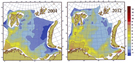Issued from: E. Eriksen, H.R. Skjoldal, H. Gjøsæter & R. Primicerio in Progress in Oceanography, 2017, 151 [p.209, Fig.3].

The Barents Sea.
Distribution of temperature (°C) at the bottom, August-September 2004 (left panel) and 2012 (right panel).

Issued from: E. Eriksen, H.R. Skjoldal, H. Gjøsæter & R. Primicerio in Progress in Oceanography, 2017, 151 [p.209, Fig.2].

Long term series (1980-2015) of annual temperature at the Fugløya-Bjørnøya section (grey line) and 10 years moving average shown with black line.

Arctic Ocean:

The North Atlantic Drift enters the Norwegian Sea between the British Isles and Iceland.
Part of it washes the southern coasts of Iceland, creating a slight westward current, while the main part reaches the coasts of Norway, carrying warm water as far as the Barents Sea, which breaks up the pack ice in summer to reach the western coast of Novaya Zemlya and the southern part of Franz Josef Land. These waters also clear the coasts of Spitsbergen every year.
From Spitsbergen onward, the saline waters of the North Atlantic Drift no longer directly affect the ocean surface, whose temperature remains low (-0.9° to -1.6°C), and whose salinity is low (< 30). But from a depth ranging from 100 to 200 metres, the warm, saline Atlantic waters are found again, with temperatures above 0° and a salinity of at least 35. It is their greater density that forces the Atlantic waters to sink beneath the polar waters. These Atlantic waters, which only travel at depth, cool as they move Eastward: North of Spitsbergen their temperature is +3° to +4°C, North of Franz Josef Land +1°C, and North of the New Siberian Islands +0.4°C. They do not reach the northern shores of Siberia, which is protected by a shallow continental shelf, covered by almost fresh, very cold water.
The North Atlantic Drift does not have the regularity of a true current and depends on the prevailing winds. As a result, it feeds the depths of the Arctic basin in a variable way from year to year.
The boundary between the cold, low-salinity surface waters and the warmer, more saline deep waters is animated by vertical oscillations (internal waves) of large amplitude.

Fram Current:
The inflow of warm, saline water from the Atlantic is offset by a cold current that begins east of the New Siberian Islands, flows Northwestward and Northward, passing near the pole, and leaves the Arctic Ocean along the eastern coast of Greenland.
In the central Arctic basin, the speed of the permanent current toward the Greenland Sea is low, less than 1 mile per day. Amundsen, during his 1925 expedition, observed, between Spitsbergen and the pole, at 88° latitude, a drift of 12 miles in 20 days toward the Southwest-Southeast, that is, roughly toward the middle of the strait separating Spitsbergen from Greenland.
On approaching the Greenland Sea, the current increases: at the 83° parallel, its speed is 2 miles per day; at 80°, it is 3 to 4 miles; at 75°, 5 miles per day.

Greenland Current:
The southward current following the eastern coast of Greenland is sustained by the North and Northwest winds that predominate in this region.

Baffin Sea Current:
On reaching Cape Farewell (the tip of the southeastern point of Greenland), the Greenland Current splits: while one part heads directly toward Newfoundland, the other moves up the western coast of Greenland for a while, before eventually merging into the Baffin Sea Current, which flows Southward from higher latitudes. An ice drift has been observed from latitude 77° to latitude 53°, covering 1500 miles in a little over 6 months.
The current then runs along the coasts of Labrador (where it is known as the Labrador Current), and carries icebergs South of Newfoundland.

Currents north of America and in the polar archipelago:
A variable current is observed in the Bering Strait, most frequently flowing Northward at a speed of 2 to 3 knots. This current reverses during North gales. The northward current is felt as far as the vicinity of Point Barrow (northern Alaska).
Around the mouth of the Mackenzie, the currents are uncertain, but it appears that, on the whole, the waters flow Eastward through the channels of the American polar archipelago, eventually reaching, via the Davis and Hudson Straits, the coasts of Labrador and Newfoundland. A branch of this current probably goes around the polar archipelago and Greenland to the North.
Branches of this current flow through the straits. The most important one crosses Smith Sound, joining the southward current of the Baffin Sea and the Davis Strait.
Evidence of the eastward drift in the channels of the polar archipelago is provided by the drift of the ''Resolute'', which, abandoned in May 1854 at the western end of Barrow Strait, was found again in September 1855 at the southern end of Davis Strait; during those 16 months, the abandoned ship had covered 1100 miles, at an average speed of 2.3 miles per day.

References:
J. Rouch, 1948. Traité d'océanographie physique. 3, pp.337-341. Édit. Payot, Paris
Atlas of Pilot Charts http://msi.nga.mil/NGAPortal/MSI.portal?_nfpb=true&_pageLabel=msi_portal_page_62&pubCode=0003 NATIONAL GEOSPATIAL-INTELLIGENCE AGENCY (USA)

 

Bipolar species

One species: Spinocalanus antarcticus is only observed in the Antarctic and in the Arctic polar basin. 49 species may be considered bipolar: Aetideopsis minor, Aetideopsis rostrata, Augaptilus glacialis, Bradyidius armatus, Chiridius gracilis, Epicalymma schmitti, Epicalymma umbonata, Euchirella rostrata, Gaetanus brevispinus, Gaetanus tenuispinus, Haloptilus acutifrons, Haloptilus longicornis, Metridia longa, Metridia lucens, Metridia princeps, Microcalanus pusillus, Microcalanus pygmaeus, Microsetella norvegica, Mimocalanus distinctocephalus, Neomormonilla minor, Oithona atlantica, Oithona similis-Group, Oncaea compacta, Oncaea englishi, Oncaea lacinia, Oncaea parila, Oncaea pumilis, Paracalanus parvus, Paraeuchaeta barbata, Paraheterorhabdus (Antirhabdus) compactus, Pleuromamma robusta, Pseudhaloptilus eurygnathus, Pseudhaloptilus pacificus, Pseudoamallothrix ovata, Pseudochirella batillipa, Pseudochirella spectabilis, Racovitzanus antarcticus, Rhincalanus nasutus, Scaphocalanus magnus, Scolecithricella minor, Spinocalanus abyssalis, Spinocalanus antarcticus, Spinocalanus elongatus, Spinocalanus horridus, Spinocalanus longicornis, Spinocalanus magnus, Talacalanus greeni, Temorites brevis, Triconia conifera.

It should be noted that some of these bipolar species are regularly carried into temperate or sub-tropical zones by the ocean currents (Aetideopsis minor, Pseudochirella spectabilis, Spinocalanus horridus, Epicalymma schmitti).

‹ Marine currentsCosmopolitanism ›